
Diagnosis of Adenocarcinomas in Histology Images Using Persistence Homology and Deep Learning
Differentiability and topological characteristics of the glandular structures is one of the key factors in the diagnosis and grading of adenocarcinomas through histology images. We believe persistent homology is an excellent mathematical tool to quantify these characteristics. In this blog post, we present a deep learning approach for encoding the glandular epithelium architecture based on a recently developed vectorized persistent homology representation called persistence images and demonstrate its application to automated diagnosis of colorectal adenocarcinomas with very encouraging results.
Introduction
Histopathology is the study of the presence, extent, and progression of a disease through microscopic examination of thin sections of biopsied tissue. These sections are chemically processed, fixed onto glass slides, and dyed with one or more stains to highlight different cellular/tissue components (e.g., cell nuclei, cell membrane, cytoplasm) and antigens/proteins (e.g., Ki-67 indicating cell proliferation). Histologic evaluation is regarded as the gold standard in the clinical diagnosis and grading of several diseases, including most types of cancer.
In clinical practice, histologic evaluation still largely depends on manual assessment of glass slides by a pathologist with a microscope. Improvements in whole-slide imaging devices and subsequent regulatory approval of whole-slide-imaging and computational algorithms, however, are rapidly paving the way for increased clinical use of digital imaging and computational interpretation. Algorithmic evaluation of tissue specimens may eventually improve the efficiency, objectivity, reproducibility, and accuracy of the diagnostic process.
One of the main challenges in automating the interpretation of histopathology images is the recognition of complex, high-level semantics to identify the presence and degree of malignancy. Recently, deep learning techniques have achieved state-of-the-art performance in several such complex visual recognition tasks in both general computer vision and medical imaging data. In contrast to traditional machine learning models, whose success relies heavily on consulting with domain experts and carefully hand-crafting discriminative features of relevance to the clinical problem, deep learning techniques are capable of automatically learning these features from the raw image data.
However, the success of deep learning models relies on the availability of a large amount of training data, which is difficult to obtain in medical domains. While techniques such as transfer learning and data augmentation can address this problem to an extent, they are not always sufficient. In such a scenario, we believe that figuring out mechanisms to incorporate domain knowledge about the clinical problem in a way that is amenable to the application of deep learning models could be helpful.

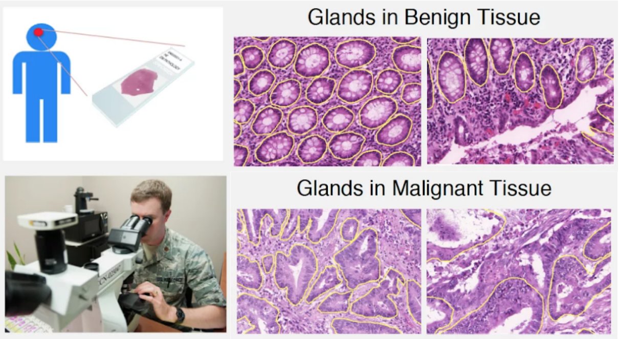
For adenocarcinomas (tumors originating in glandular structures of epithelial tissue such as prostate, pancreatic, and colorectal cancers), the differentiability of glandular architecture in histopathology images is one of the key criteria used by pathologists to determine the presence and degree of malignancy (Figure 1). Normal-appearing structures with organized epithelium become disorganized with the unchecked growth and aberrant signaling typical of cancer.
We believe persistent homology is an excellent mathematical tool to quantify such complex characteristics about the topology and architecture of the glandular structures. In a prior blog post, we reported promising preliminary results on a small dataset indicating that a traditional machine learning model called random forest trained on two recently developed vectorized persistence homology representations called persistence landscapes and persistence images can be effective in discriminating between benign and malignant colorectal cancer from histology images. In this blog post, we investigate the effectiveness of advanced deep convolutional neural network (CNN) models trained on both raw RGB and persistence images in the diagnosis of colorectal cancer from a relatively larger set of histology images.
Background on Persistent Homology
Given a point cloud dataset, persistent homology can be seen as a theoretical tool to detect and characterize prominent topological features (e.g., connected components, loops, voids) at multiple scales [7]. In this section, we present a brief background on some fundamental concepts of persistent homology and the two recently proposed vectorized persistent homology representations called persistence landscapes and persistence images. See our prior blog post for a more detailed coverage of these concepts.
- Simplex: A p-simplex σp is defined as the convex hull of p+1 affinely independent points / vertices. A face of a simplex is defined as a subset of its p+1 points/vertices.
- Simplicial complex: A simplicial complex K is a finite collection of simplices. If a simplex is in K then all its faces are in K. Given a simplicial complex K, a simplicial complex L formed by a subset of its simplices is referred to as the sub-complex of K denoted as 𝐿 ⊂ 𝐾.
- Filtration: A nested sequence of simplicial complexes 𝜙 ⊂ 𝐾1 ⊂ 𝐾2 ⊂ ⋯ ⊂ 𝐾n = 𝐾 is called a filtration of K.
- Homology groups: A d-dimensional homology group Hd(K) of a simplicial complex K is the set of all d-dimensional voids in K and the rank or number of these voids is referred to as the d-dimensional Betti number 𝛽d(𝐾).
- Vietoris-Rips Filtration: Given a point set, a simplicial complex VR 𝜎 = {𝜎 ∣ 𝑑𝑖𝑎𝑚 𝜎 ≤ 𝜖} containing simplices of all subsets of its points whose max distance < 𝜖 is called a Vietoris-Rips (VR) complex. An increasing sequence of diameters/scales 𝜖1 < 𝜖2 < ⋯ < 𝜖n results in a nested sequence of VR complexes 𝑉𝑅(𝜖1) ⊂ 𝑉𝑅(𝜖2) ⊂ ⋯𝑉𝑅𝜖n) known as the Vietoris-Rips (VR) Filtration.
- Persistence diagram: Given a filtration F, the idea of persistent homology is to track the scales at which each d-dim void appears/disappears as a multiset 𝐵𝐷d = {(𝑏i, 𝑑i)} of birth-death scales. Plotting them as 2D points produces the persistence diagram (PD) representation. This summarization of topological information as a multiset of points is not amicable for machine learning models such as RandomForest, XGBoost, and Neural Networks wherein a vectorized representation is more convenient [10]. Persistence landscapes [10] and persistence images [6], described below, are two recently developed vectorized persistent homology representations to address this problem (Figure 2).
- Persistence landscape: Given a multiset of birth-death pairs { (bi, di) } with a triangular shaped function 𝑓i(𝑥) that linearly increases from (bi,0) to ( (𝑏i+di)/2, (bi+di)/2 ) and then linearly decreases until (di, 0), the persistence landscape is defined as a 2D function 𝜆:𝑁 𝑥 𝑅→[0, ∞] where 𝜆(𝑘,𝑥) is k-th largest value of { 𝑓i(x) }.
- Persistence image: Given a multiset of birth-persistence values 𝐵𝐷d(𝐹)={(𝑏i, 𝑝i)} of all d-dim voids, the persistence image (PI) representation is generated by discretizing a 2D real-valued function defined as a weighted sum of bivariate gaussian PDFs centered at each birth persistence pair as follows: ρ(x, y) = Σiw(bi, pi) x N(x-bi, y-pi;σ2). One of the main advantages of persistence images over persistence landscapes is that persistence images lie in Euclidean space and hence are more amenable to a wide variety of machine learning techniques. They are also easier to interpret than persistence landscapes due to their close resemblance to the persistence diagram.

Methodology
In this section, we present our approach for the diagnosis of adenocarcinomas from histopathology images using deep learning and persistence homology.
Detect nuclei centroids: Given a histology image, we first pre-process it using the color normalization method of Reinhard et al [9] to standardize the staining. Next, we use the unsupervised color deconvolution method of Macenko et al [3] to extract the nuclear stain and apply minimum cross entropy thresholding [4] to segment the nuclear foreground. Lastly, we use a fast Difference-of-Gaussian implementation of a scale-adaptive Laplacian-of-Gaussian of Al-Kofahi et al [5] filter to detect nuclei centroids. The aforementioned pipeline of methods were developed using their implementations in HistomicsTK: an open-source Python toolkit for histopathology image analysis that we are actively developing.
Characterization of glandular topology using persistence images: Considering the set of nuclear centroids as a point cloud, we compute the persistence diagram of its Vietoris-Rips filtration for the homological dimension-1 corresponding to 2D loops using a fast multiscale approach developed at Kitware [2]. We then compute the persistence image representation of this persistence diagram to characterize the 2D voids/loops formed by the point set of glandular epithelial cell nuclei at multiple scales (Figure 3).

Training deep learning models for cancer diagnosis: Given a training set of benign and malignant images, we investigated three different deep learning methodologies: (i) CNN trained on raw RGB images, (ii) CNN trained on persistence images, and (iii) a two-stream CNN trained on both RGB and persistence images. Further details about each of these models are given below.
- RGB model: We chose to use ResNet50 CNN architecture, which produced state-of-the-art performance on the ImageNet dataset, as the base network for the RGB model. ResNets introduced the notion of residual / identity-shortcut / skip connections that allow us to effectively train deeper networks without running into the vanishing gradient problem. For our RGB model, we use the convolutional part of the ResNet50 architecture and Global Average Pool the output to obtain a 2048 dimensional feature vector. This is followed by a dense layer of size 128 which is then fed to a softmax classification with 2 neurons. ReLU activation is used following the Global Average Pooled and the dense layer and dropout (probability 0.3) is used for regularization. The weights of the base network are initialized from ResNet50 weights pre-trained on ImageNet. A schematic of the RGB model is shown in Figure 4.
- Persistence Model: The persistence model takes in a single channel persistence image as input which is followed by two convolutional layers. The output is global average pool followed by a dense layer of size 128. This feature vector is then fed to a softmax classification layer with 2 neurons. Batch-normalization is used following the two convolutional layers which helps keep the intermediate layers normalized and avoid internal covariance shift. In addition, drop-out (probability=0.3) is also used after each dense layer. A schematic of the persistence model is shown in Figure 5.
- Hybrid Model: The hybrid model is constructed by combining the both the RGB and the persistence models. Specifically, the features extracted by final dense layers of both the RGB and persistence sub-models are concatenated and then fed to a softmax classification layer. A schematic of the hybrid model is shown in Figure 6.


Results
We used the colon cancer dataset provided by [1]. This dataset contains H&E stained histopathology images collected from the Department of Pathology of Zhejiang University in China that are scanned using the NanoZoomer slide scanner from Hamamatsu. Regions containing typical cancer subtype features are cropped and selected following the review process by three histopathologists, in which two pathologists independently provide their results and the third pathologist merges and resolves any conflict in their annotations. It contains images of a total of 717 regions (355 malignant, 362 benign) with a maximum scale of 8.51×5.66 mm and average size of 5.10mm2. All images were obtained at 40x magnification with a resolution of 226 nm/pixel. We create our training dataset by dividing these images into patches of size 1024×1024 with an overlap of 128 pixels and assign the image label to all the patches extracted from each image. Note that this may not always be true as there could be benign patches inside a malignant image. However, this was the best public, labeled dataset that we could find. We assume that the deep learning models can be resilient to such noisy labels provided that they do not occur very frequently in the dataset.
Data preprocessing: Many of the patches in the dataset turn out to be low contrast images, contain a significant amount of background and/or tissue regions with very few nuclei. We discard such patches based on the following three criteria:
- Low contrast: We compute the upper percentile (99%) and the lower percentile (1%) of the intensity values from the image. An image is considered low contrast if its range of brightness falls below a fraction (0.05) of the data type’s maximum intensity value (255 in our case).
- Significant amount of background: As a first pass, we calculate the percentage of pixels whose RGB channel values are all greater than or equal to 200. If this percent is greater than 70% (i.e., the image has mainly white background), the image is rejected. As a second pass, we use a two-component Gaussian mixture model to compute a binary mask separating the tissue areas from background in brightfield H&E images. The image is rejected if the foreground is less than 30% of the image area.
- Low nuclear count: We first standardize the staining using a color normalization method [9], then extract the nuclei stain using a supervised color deconvolution method. Next, nuclear foreground mask is extracted by thresholding and morphology operations. The image is rejected if the foreground is less than 10% of the image area.
The remaining images are then split into train, validation, and test sets. We made sure that all the patches from a single image are included in only one of these three sets to avoid similar looking images. The final distribution of the data after the split is shown in Table 1 below:

Training: It is clear from Table 1 that the training data is skewed towards malignant samples. This will make the model biased towards predicting a malignant class more often than a benign class. We use inverse weight balancing to mitigate this issue of class imbalance, where the loss is multiplied by a certain factor inversely proportional to the frequency of the number of samples from that class. All the models were implemented in Keras with a TensorFlow backend. If the validation loss does not decrease after 2-3 epochs, we use the Adam optimizer and reduce the learning rate by a factor of 2. All the models were trained with a categorical cross entropy loss. The model weights are saved to a checkpoint by monitoring the validation loss. The RGB image is preprocessed by subtracting from it the individual means for three channels and dividing them by the variances, both of which are obtained from the ImageNet dataset. The persistence images are scaled by dividing each pixel value by a factor which is calculated as the 95th percentile of all the persistence images in the training set.
We first trained the RGB and persistence models individually. The RGB model was initialized using ResNet50 weights trained on ImageNet whereas the persistence model was randomly initialized.The respective submodels of the hybrid model were initialized from the best checkpoints obtained from the previous step. Table 2 shows a comparison of the performance from the various models.


Figures 7 and 8 show the False Positive and False Negative samples from the test set, respectively. Of the total 1026 samples used for testing, the hybrid model had a false negative count of 21 and a false positive count of 160. This shows that many of the benign patches are being classified as malignant which might be due the label noise introduced by assigning the image level label to all the patches extracted from it.
Conclusion
In this work, we investigated the use of deep learning and persistence homology for the diagnosis of adenocarcinomas in histology images. Our results indicate that a deep learning model trained on raw RGB images performs significantly better than persistence images. While the hybrid model produces the best performance amongst the three, but contrary to our expectation, it performs only slightly better than the model trained on raw RGB images. This suggests that the hybrid model is able to extract information very similar to that obtained from raw RGB images. Also, the performance of even the best model is lower than expected, probably due to the assignment of image-level labels to all of its patches which might be inducing a significant amount of label noise in the dataset. In the future we plan to use multiple instance learning [8] to address this problem. The source code for this project is in this GitHub repository: https://github.com/KitwareMedical/HistologyCancerDiagnosisDeepPersistenceHomology.
Acknowledgements
This work was funded by the NIH ITCR U01 grant 1U01CA220401-01A1 entitled “Informatics Tools for Quantitative Digital Pathology Profiling and Integrated Prognostic Modeling” with Dr. Lee Cooper (Emory University), Dr. Metin Gurcan (Wake Forest School of Medicine), and Dr. Christopher Flowers (Emory University) as PIs and Kitware as a subcontractor.
References
- Y. Xu, Z. Jia, L.-B. Wang, Y. Ai, F. Zhang, M. Lai, E.I.-C. Chang, Large scale tissue histopathology image classification, segmentation, and visualization via deep convolutional activation features, BMC Bioinform. 18 (2017) 281.
- S. Gerber, “Fast approximate multiscale persistence homology computation”, https://bitbucket.org/suppechasper/homology
- M. Macenko, M. Niethammer, J. S. Marron, et al., “A method for normalizing histology slides for quantitative analysis,” in IEEE International Symposium on Biomedical Imaging: From Nano to Macro, June 2009, pp. 1107–1110.
- H. Li and P.K.S. Tam, “An iterative algorithm for minimum cross entropy thresholding,” Pattern Recognition Letters, vol. 19, no. 8, pp. 771–776, June 1998.
- Y. Al-Kofahi, W. Lassoued, W. Lee, et al., “Improved automatic detection and segmentation of cell nuclei in histopathology images,”IEEE Transactions on Biomedical Engineering, vol. 57, no. 4, pp. 841–852, 2010
- H. Adams, et al., “Persistence Images: A Stable Vector Representation of Persistent Homology,” JMLR, 18(1), 2015.
- X. Zhu, “Persistent homology: An introduction and a new text representation for natural language processing,” in IJCAI, 2013.
- M.A. Carbonneau, V. Cheplygina, E. Granger, and G. Gagnon. (2016). “Multiple instance learning: A survey of problem characteristics and applications.”
- E. Reinhard, M. Ashikhmin, B. Gooch, et al., “Color transfer between images,”IEEE Computer Graphics and Applications, vol. 21, no. 5, pp. 34–41, 2001.
- P. Bubenik, “Statistical topological data analysis using persistence landscapes,” JMLR, 16(1), 2012.