
Post-processing visualization of high-order solutions using the Gmsh Reader plugin in ParaView
Introduction
Recently high-order finite element methods initially introduced in the research community such as discontinuous Galerkin (DG) [7, 5, 6] and flux reconstruction (FR) [10, 14, 15] have gained considerable attention in industry, thanks to their high-accuracy on unstructured meshes, their efficiency and scalability. However, the lack of visualization tools able to handle a large number of degrees of freedom (dof) has been a major bottleneck for the analysis of high-order finite element solutions generated by massively parallel simulations.
The open source mesh and visualization tool Gmsh [9] provides a general method for the post-processing of high-order finite element fields [12]. This method relies on recursive h-refinements of the initial mesh, coupled to a projection error estimation. The high-order solution is then interpolated at the new mesh nodes in order to provide an optimal visualization grid. However, Gmsh is in essence a serial tool and is therefore limited to a relatively low number of dof and level of h-refinements.
On the other hand, ParaView [1] is an efficient open source parallel visualization tool which has been used successfully for post hoc visualization of large scale, unstructured data sets up to several billions of dof. However, ParaView relies on the Visualization Toolkit (VTK) [13] whose data models have historically mainly supported linear elements. Only very recently, arbitrary-order Lagrange polynomials have been introduced in VTK and their support in ParaView [8] for both high-order meshes and solutions is gaining traction, which confirms the growing interest and need for such features.
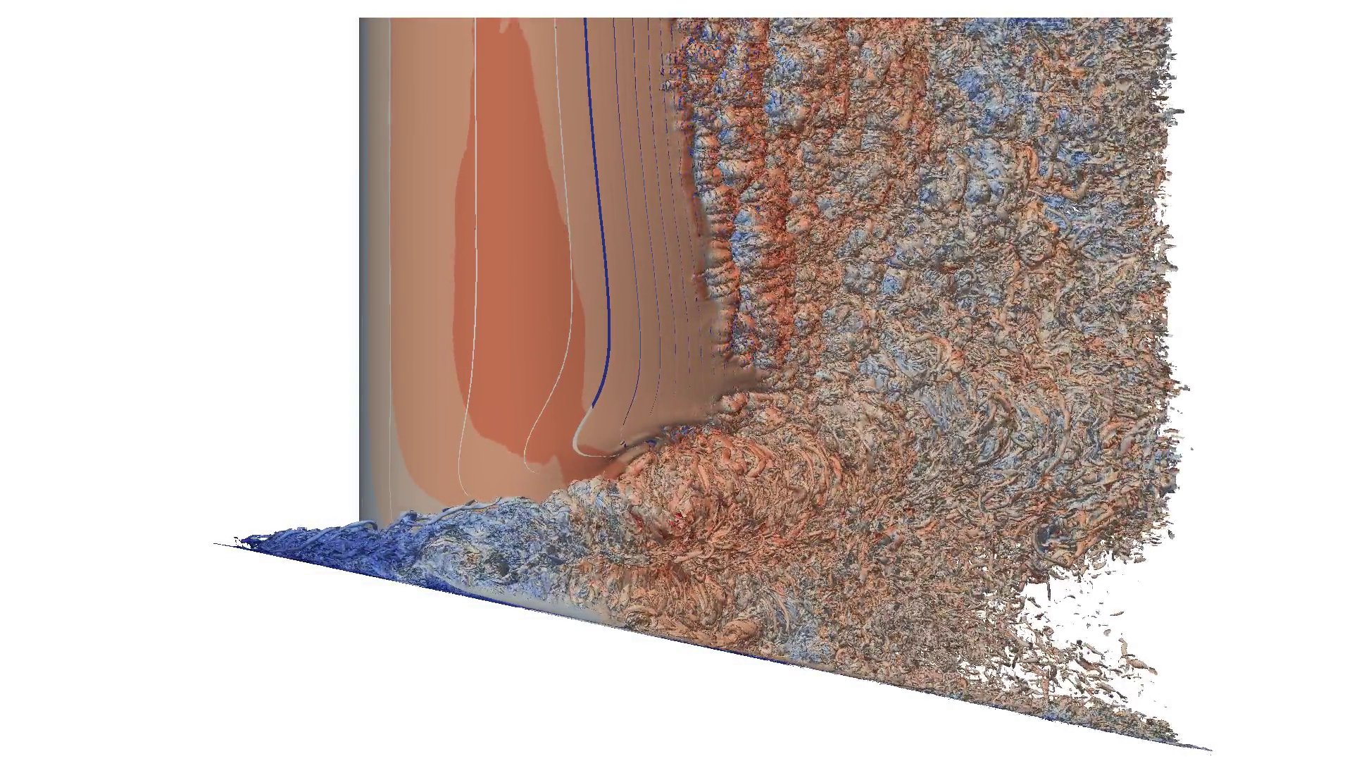
In this context, a new ParaView plugin which integrates Gmsh as an external library has been implemented for off-line post-processing and visualization of high-order solutions saved under the Gmsh format, see Figure 1. This plugin combines respectively ParaView’s scalability in parallel and Gmsh’s ability to apply h-refinement of the initial mesh followed by the interpolation of any arbitrary high-order polynomial solutions on the resulting visualization grid. This coupling enables parallel visualization of massive high-order solution in parallel, in client-server mode.

Features and implementation
Historically, few open source tools provide high-order meshing and visualization capabilities. Gmsh belongs to this category. Moreover, a major asset of the native file format of Gmsh consists in the use of an explicit description of the polynomial basis functions within the file, instead of an imposed convention. This allows to encode any polynomial basis using the same framework. The visualization capabilities of Gmsh rely on a two-step strategy further described in [12]. First, a recursive h-refinement of high-order elements based on classical automatic mesh refinement (AMR) is applied and defines a refined linear visualization grid. Then, the high-order polynomial solution is interpolated on the new nodes of the refined visualization grid. Afterwards, traditional visualization of the solution occurs through a straightforward piecewise linear interpolation on the
refined visualization grid.
The recursive h-refinement of the initial mesh which generates the visualization grid can be either uniform (every edge of the parent element is split in the same way) or selective, based on a local visualization error. In the second case, recursive h-refinements is applied to the parent elements and their child elements until this error is locally minimized. Consequently, memory requirement can be significantly reduced for the selective h-refinement procedure compared to uniform h-refinement.
Recently, the support for arbitrary-order Lagrange polynomials has also been introduced in ParaView [8]. Although it has not been tested yet within this work, this new feature opens up additional promising perspectives for the visualization of high-order meshes and solutions. Note that contrary to Gmsh, VTK supports exclusively Lagrange polynomials and ParaView provides uniform h-refinement to visualize these polynomials.
The resulting new ParaView plugin named “GmshReader” is now provided with the official ParaView source code (version 5.7.0 and above). Note that this plugin is not provided in the binary release of ParaView. In order to be able to use this plugin, one requires to compile a light version of Gmsh compiled as an external library as well as compiling ParaView itself with the plugin enabled. See here for more information. In order to limit its memory consumption, this light version of Gmsh only embarks the internal data reader and the visualization procedure described above and customized for this particular application. Consequently, this plugin uses the same h-refinement and interpolation procedures as in Gmsh to generate a refined visualization grid. This visualization grid follows a linear VTK data format that is passed to ParaView for linear visualization. Further details of this implementation can be found in [11].
Illustration
The examples shown in this section have been generated with the massively parallel high-order discontinuous Galerkin CFD code named Argo developed at Cenaero [4, 3, 2] but the tools and approaches presented in this blog can be applied to any high-order polynomial data set.
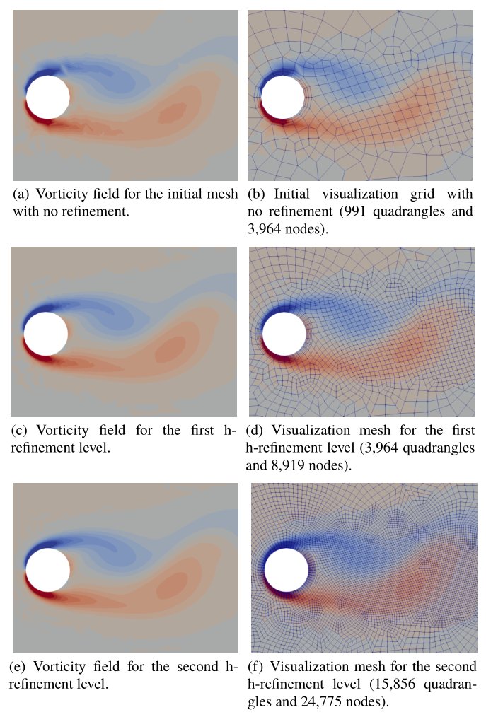
The capability of the GmshReader plugin is first illustrated in Fig. 2 with the 2D flow past a circular cylinder at Reynolds number 100. The initial mesh includes 991 second-order quadrangles whereas the solution field is represented by fourth-order p4 Lagrange polynomials, which leads to a total of 24,775 dof per equation with 25 dof per equation per quadrangle. The fourth-order Lagrange p4 vorticity field is shown in the left panels of Figure 2 whereas the associated visualization grids are shown in the right panels for several uniform h-refinement levels of the initial mesh.
As shown in Fig. 2, two levels of h-refinement are typically sufficient to ensure a proper level of convergence for the considered field. In this example, two levels of uniform h-refinement results in 15,856 linear quadrangles and 24,775 nodes in the visualization grid. Note that the number of linear quadrangles and nodes could have been further reduced if selective h-refinement had been applied for the visualization of this single field. Other examples with selective h-refinement are provided in [12].
The linear representation of the cylinder geometry is also improved as the number of h-refinement levels increases, which highlights the projection of the new mesh nodes on the boundary surfaces that occurs in Gmsh after each h-refinement.
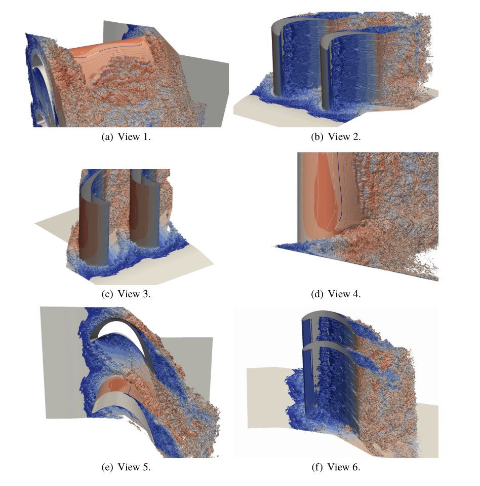
As a second example, the visualization of the 3D flow field around the full span MTU T161 low pressure turbine blade cascade is illustrated in Fig. 3 with six views of a vorticity isosurface pseudo-colored by velocity magnitude. This test case includes 14.9 million hexahedra partitioned in 4,800 mesh parts and the solution is represented by third-order p3 Lagrange polynomials, leading to about 0.96 billion dof per equation. Two levels of h-refinement are applied in Fig. 3. The visualization system Cooley located at the Argonne Leadership Computing Facility was used for these tests.
Conclusions
An open source ParaView plugin named GmshReader has been implemented for the parallel visualization of any arbitrary high-order polynomial solution saved under the Gmsh native format. This plugin combines the assets of both ParaView and Gmsh, which are the scalability and rich library of available data operations for the former, and a flexible representation of any high-order polynomial function for the latter. The visualization approach implemented in Gmsh relies on the recursive h-refinement of the initial mesh to generate a refined visualization grid, followed by the interpolation of the high-order solution on the visualization grid. The h-refinement in Gmsh can be uniform or selective based on a local visualization error, although the selective h-refinement is currently limited to the processing of a single field whereas multiple fields can be handled simultaneously with uniform h-refinement. The resulting visualization grid and associated interpolated solution can then be efficiently visualized with ParaView.
As future improvement, uniform h-refinement in Gmsh currently relies on the same recursive algorithm as local h-refinement based on a local visualization error and is consequently applied on an element per element basis. Instead, uniform h-refinement could perform efficient projection of the high-order solution on the visualization grid using BLAS functions. Indeed the projection matrix which stores the values of the shape functions at the nodes of the visualization grid pattern is constant in the parametric space of all elements of the same topology and could therefore be recycled.
Then, the recent introduction of arbitrary high-order Lagrange polynomials in VTK and their support in ParaView pave the way to further CPU time and memory requirements reduction for the visualization of high-order solutions. Although ParaView currently relies on uniform h-refinement of high-order meshes, only the elements directly involved in a given data operation could be selectively refined in the future (e.g. elements intersected by a slice or an isosurface), reducing significantly the memory consumption.
Finally, for post hoc visualization with the GmshReader plugin, uniform h-refinement specifically applied to Lagrange elements could be further accelerated in ParaView compared to the current flexible and recursive algorithm based on a local visualization error in Gmsh.
Acknowledgements
In addition to the TILDA H2020 grant, this work was partially funded by a Beware fellowship from the Walloon Region of Belgium under grant agreement No 1410131.
Another award of computer time used for this work was provided by the Innovative and Novel Computational Impact on Theory and Experiment (INCITE) program. This research used the visualization resource Cooley of the Argonne Leadership Computing Facility, which is a DOE Office of Science User Facility supported under Contract DE-AC02-06CH11357.
The present research benefited from computational resources made available on the Tier-1 supercomputer of the federation Wallonie-Bruxelles, infrastructure funded by the Walloon Region under the grant agreement n1117545.
Last but not least, Mathieu Westphal and Joachim Pouderoux from Kitware are gratefully acknowledged for their help to integrate the plugin in the ParaView sources.
References
1. James Ahrens, Berk Geveci, and Charles Law. Paraview: An end-user tool for large data visualization. The visualization handbook, 717, 2005.
2. C. Carton de Wiart and K. Hillewaert. A discontinuous Galerkin method for implicit LES of moderate Reynolds number flows. In AIAA SciTech, 53rd AIAA Aerospace Sciences Meeting, Kissimmee, Florida, January 2015.
3. C. Carton de Wiart, K. Hillewaert, L. Bricteux, and G. Winckelmans. Implicit LES of free and wall bounded turbulent flows based on the discontinuous Galerkin/symmetric interior penalty method. International Journal of Numerical Methods in Fluids, 78(6):335–354, 11 March
2014. doi 10.1002/fld.4021.
4. C. Carton de Wiart, K. Hillewaert, M. Duponcheel, and G. Winckelmans. Assessment of a discontinuous Galerkin method for the simulation of vortical flows at high Reynolds number. Int. J. Numer. Meth. Fluids, 74:469–493, 2013. doi: 10.1002/fld.3859.
5. Bernardo Cockburn. Discontinuous galerkin methods for convection-dominated problems. In High-order methods for computational physics, pages 69–224. Springer, 1999.
6. Bernardo Cockburn, George E Karniadakis, and Chi-Wang Shu. The development of discontinuous galerkin methods. In Discontinuous Galerkin Methods, pages 3–50. Springer, 2000.
7. Bernardo Cockburn and Chi-Wang Shu. The local discontinuous galerkin method for time-dependent convection-diffusion systems. SIAM Journal on Numerical Analysis, 35(6):2440–2463, 1998.
8. Thomas J Corona and David Thompson.
Arbitrary-order lagrange finite elements in the visualization toolkit. Kitware Source Quaterly Magazine, 43:6–9, 2018.
9. Christophe Geuzaine and Jean-François Remacle. Gmsh: A 3-d finite element mesh generator with built-in pre-and post-processing facilities. International journal for numerical methods in engineering, 79(11):1309–1331, 2009.
10. Hung T Huynh. A flux reconstruction approach to high-order schemes including discontinuous galerkin methods. In 18th AIAA CFD Conference, page 4079, 2007.
11. M. Rasquin, A. Bauer, and K. Hillewaert. Scientific post hoc and in situ visualisation of high-order polynomial solutions from massively parallel, simulations. International Journal of Computational Fluid Dynamics, 33(4):171–180, 2019.
12. Jean-François Remacle, Nicolas Chevaugeon, Emilie Marchandise, and Christophe Geuzaine. Efficient visualization of high-order finite elements.
International Journal for Numerical Methods in Engineering, 69(4):750–771, 2007.
13. Will J Schroeder, Bill Lorensen, and Ken Martin. The visualization toolkit: an object-oriented approach to 3D graphics. Kitware, 2004.
14. David M Williams, Patrice Castonguay, Peter E Vincent, and Antony Jameson. Energy stable flux reconstruction schemes for advection–diffusion problems on triangles. Journal of Computational Physics, 250:53–76, 2013.
15. FD Witherden, PE Vincent, and A Jameson. High-order flux reconstruction schemes. In Handbook of Numerical Analysis, volume 17, pages 227–263. Elsevier, 2016.