
HyperTreeGrid in VTK: An introduction
This is the first part of a series of blog articles about vtkHyperTreeGrid usage and implementation in VTK. The second part, HTG data construction, can be found here, the third part, HTG: Using Masks, can be found here, the fourth part, HTG: Specific Filters, can be found here, the fifth part, HTG: Cursors and Supercursors, can be found here.
To optimize the usage of available ressources, Adaptive Mesh Refinement (AMR) techniques focus the computational effort and memory usage where they are needed.
Codes using these AMR techniques are particularly effective at tracking fine details in areas of interest while remaining coarse elsewhere. This offers a good compromise between numerical precision, memory footprint and calculation cost, by proposing to preserve, refine or coarse a region during the simulation. In addition to the requirement for significant re-engineering of both algorithms and codes, the main difficulties in AMR techniques lie in the definition of the refinement criteria and especially coarsening.
Without going into more detail on the pros and cons, the benefits are particularly highlighted in cosmological simulations, which can reach tens of billions of fine cells / leaves of interest for the most recent ones [1].
Since the first description of AMR techniques by Berger-Oliger-Colella in the ‘80s, several implementations have been proposed and developed, in particular:
- based-blocks AMR or patch-blocks AMR or AMR structured by blocks or corrective AMR,
- tree-based AMR (TB-AMR) or even point-structured AMR.
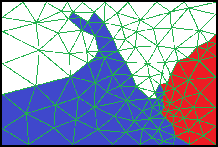
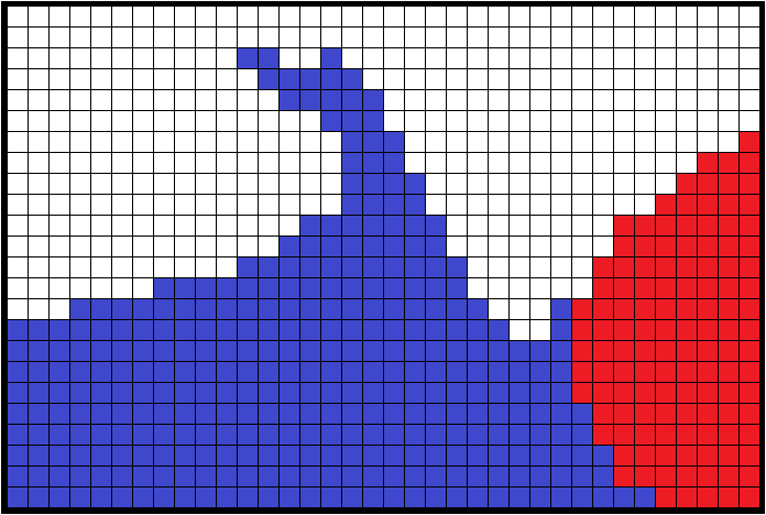
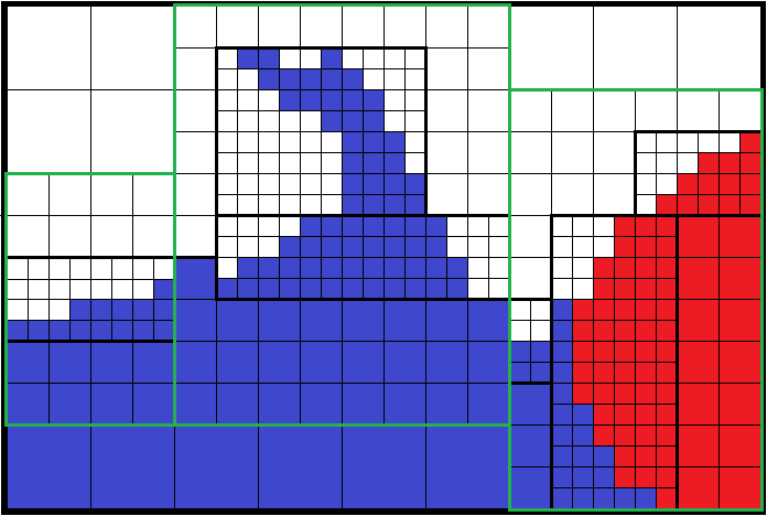
| unstructured | structured | block-based AMR | tree-based AMR | |
|---|---|---|---|---|
| Data structure complexity | simple | very simple | simple | complex |
| Accuracy | very high | can be high* | can be high* | can be high* |
| Traversal complexity | high | low | low** | low** |
| Geometry storage | very high (~2ku) | very low (~9u) | very low (~90u) | low (25u-~200u)*** |
| Quantity storage | low (~200u) | very high (~800u) | high (~400u) | low (~200u) |
* The accuracy can be improved by associating the description of an interface for each mesh (one or two parallel planes faces). This is expensive, but optional.
** The traversal could be improved by exploiting the hierarchical description. Reducing the smoothness of the results will also reduce the loading time.
*** Could be reduced depending on the storage mode.
In comparison with the first implementation, for a simulation taking advantages of AMR techniques, the second implementation will have a better memory usage but an increased complexity in writing algorithms which, at first glance, would not support vectorization. This dichotomy between these methods stems from the more general opposition between implicit and explicit representations.
Beyond the simulation code aspect, the analysis and visualization aspect in VTK is addressed for the TB-AMR (Tree-Based Adaptive Mesh Refinement) implementation through the HyperTreeGrid representation. Thanks to the vtkResampleToHyperTreeGrid filter of the ParaView HyperTreeGridADR plugin, it is possible to build a HyperTreeGrid representation from many representations available in VTK.
One of the advantages is the acceleration of the exploration by limiting the display in depth as in the search for hot spots. This approach is only possible if the maximum value reached by its daughters has been associated with each coarse cell.
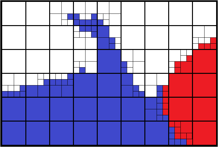
This representation consists in describing a rectilinear grid of refined trees where each element of this grid can be:
- undefined ;
- a leaf cell (a non-refined tree) ;
- a root cell of a tree, a coarse cell (a refined tree).
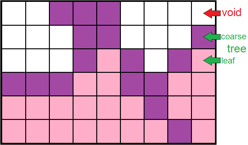
The branch factor (bf) describing the refinement is the same for all spatial directions and for all trees of the grid. In the example below, the implemented value is 2 and 3. A mesh refinement necessarily generates all the daughters (in 3D, bf=2: 8).
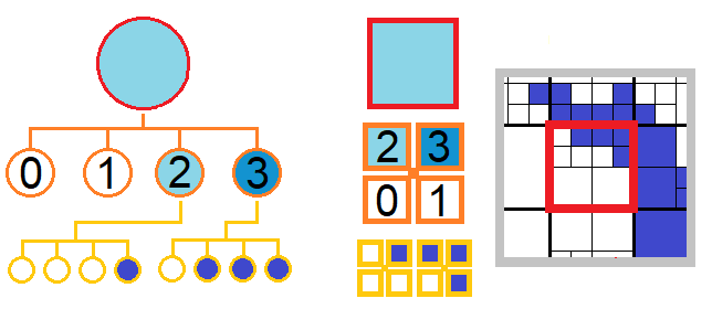
The case of a rectilinear grid reduced to only one refined tree, in 3D with bf=2 describes an octree.
A value of type, masked, or not masked, can be positioned on each cells. If a coarse cell is masked, its daughters are treated as such (although this is not explicitly so!).
In this representation, the coarse meshes are explicitly described and will carry a value for all the defined fields of values. For a controlled memory overhead (i.e. 3D, bf=2, max overhead 15%), the definition of the coarse cells will be used in order to accelerate the filters execution.
The value fields are given in the center of the cells (leaf or coarse). In this representation, it is not possible to define values at points. A filter computes, through an operator, the value associated with a coarse cell with respect to the value of its children.
The navigation through this representation is facilitated by specific iterators for cells: the cursors and the super-cursors. Cursors are associated to the information access on the current cell as well as to traversal services. The super-cursors add informations on neighboring meshes according to two patterns: Von Neuman (i.e. 3D, 6 neighbors) or Moore (i.e. 3D, 26 neighbors). The cost of traversing a mesh is directly linked to the complexity of the cursor / super-cursor selected.
On the HTG, it is possible to define:
- an indirection table dissociating how to build the HTG and the values associated with each cell;
- sub-cell informations making it possible to describe an interface.
The use of this representation requires some logic:
- choose to keep the mesh as input and only redefine the mask (as the threshold filter);
- decide to stay as long as possible in this representation (as the cut axis filter which returns a 2D HTG);
- select the most suitable cursor (as coarse evaluate filter);
- opt for a two-pass construction: a quick preset cursor before using a expensive super-cursor (as the iso-contour filter).
For the moment, the parallel distribution on servers is based on the filter of ghosts cells generation which considers that the distribution is based on the unique and complete distribution of each of the trees. This is a requirement for the HTG construction, otherwise, veiled artifacts will appear under certain conditions.
We propose to present the HyperTreeGrid representation through a serie of articles starting with the base, i.e. the construction of a mesh. The examples will be given in the form of Python instructions, easily transcribed into compiled language. The advantage of Python is to accelerate learning through experimentation.
[1] Formation of compact galaxies in the Extreme-Horizon simulation Chabanier, Bournaud & all https://www.aanda.org/articles/aa/full_html/2020/11/aa38614-20/aa38614-20.html
CEA, DAM, DIF, F-91297 Arpajon, France