Streaming in VTK : Time

With this blog, I am starting another series. This time we will cover streaming in VTK. In this context, we define streaming as the process of sequentially executing a pipeline over a collection of subsets of data. Example of streaming include streaming over time, over logical extents, over partitions and over ensemble members. Streaming belongs to set of techniques referred to as out-of-core data processing techniques. Its main objective is to analyze a dataset that will not fit in memory by breaking it into smaller pieces and processing each piece sequentially.
In this article, I will cover streaming over time. In future ones, we will dig into other types of streaming. I am assuming that you understand the basics of how the VTK pipeline works including pipeline passes and using keys to provide meta-data and to make requests. If you are not familiar with these concepts, I recommend checking out my previous blogs, specially [1], [2] and [3].
Problem statement
Let’s look at a flow-field defined over a 2D uniform rectilinear grid. We will pick a viscous flow that has a known closed-form solution so that we don’t have to write a solver. I chose a problem from my favorite graduate level fluid mechanics book: Panton’s “Incompressible Flow”. From section 11.2, flow over Stoke’s oscillating plate is a great example. Without getting into a lot of details, the solution for this problem is as follows.

This is a nice flow-field to study because it is very simple but is still time variant. This profile looks as follows (click to animate):
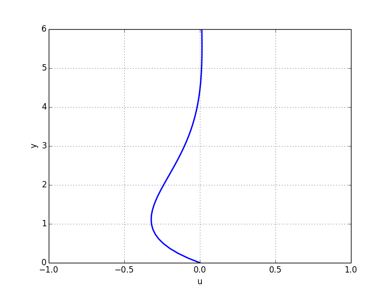
The code I used to generate this animation is here.
Source
Let’s codify this flow field as a VTK source. Even though, the flow field is really 1D (function of y only), we’ll use a 2D uniform grid (vtkImageData) such that we can advect particles later to further demonstrate temporal streaming.
import numpy as np
import vtk
from vtk.numpy_interface import dataset_adapter as dsa
from vtk.util.vtkAlgorithm import VTKPythonAlgorithmBase

t = np.linspace(0, 2*np.pi, 20)

class VelocitySource(VTKPythonAlgorithmBase):
  def __init__(self):
    VTKPythonAlgorithmBase.__init__(self,
        nInputPorts=0,
        nOutputPorts=1, outputType='vtkImageData')

  def RequestInformation(self, request, inInfo, outInfo):
    info = outInfo.GetInformationObject(0)

    info.Set(vtk.vtkStreamingDemandDrivenPipeline.WHOLE_EXTENT(),
        (0, 60, 0, 60, 0, 0), 6)

    info.Set(vtk.vtkStreamingDemandDrivenPipeline.TIME_STEPS(),
               t, len(t))
    info.Set(vtk.vtkStreamingDemandDrivenPipeline.TIME_RANGE(),
             [t[0], t[-1]], 2)

    info.Set(vtk.vtkAlgorithm.CAN_PRODUCE_SUB_EXTENT(), 1)

    return 1

  def RequestData(self, request, inInfo, outInfo):
    info = outInfo.GetInformationObject(0)
    # We produce only the extent that we are asked (UPDATE_EXTENT)
    ue = info.Get(vtk.vtkStreamingDemandDrivenPipeline.UPDATE_EXTENT())
    ue = np.array(ue)

    output = vtk.vtkImageData.GetData(outInfo)

    # Parameters of the grid to produce
    dims = ue[1::2] - ue[0::2] + 1
    origin = 0
    spacing = 0.1

    # The time step requested
    t = info.Get(vtk.vtkStreamingDemandDrivenPipeline.UPDATE_TIME_STEP())

    # The velocity vs y
    y = origin + spacing*np.arange(ue[2],  ue[3]+1)
    u = np.exp(-y/np.sqrt(2))*np.sin(t-y/np.sqrt(2))

    # Set the velocity for all points of the grid which
    # has of dimensions 3, dims[0], dims[1]. The first number
    # is because of 3 components in the vector. Note the
    # memory layout VTK uses is a bit unusual. It's Fortran
    # ordered but the velocity component increases fastest.
    a = np.zeros((3, dims[0], dims[1]), order='F')
    a[0, :] = u

    output.SetExtent(*ue)
    output.SetSpacing(0.5, 0.1, 0.1)

    # Make a VTK array from the numpy array (using pointers)
    v = dsa.numpyTovtkDataArray(a.ravel(order='A').reshape(
                dims[0]*dims[1], 3))
    v.SetName("vectors")
    output.GetPointData().SetVectors(v)

    return 1
This example is mostly self-explanatory. The pieces necessary for temporal streaming are as follows.
- Lines 20-23: This is where the reader provides meta-data about the values of time steps that it can produce as well as the overall range. The overall range is redundant here but it is required because VTK also supports sources that can produce arbitrary (not discrete) time values as requested by the pipeline.
- Line 43: The reader has to respond to the time value requested by downstream using the UPDATE_TIME_STEP() key.
If you are not familiar with VTK’s structured data memory layout, line 54 may look a little odd. VTK uses a Fortran ordering for structured data (i is the fastest increasing logical index). At the same time, VTK interleaves velocity components (i.e. velocity component index increases fastest). So a velocity array would like this in memory u_0 v_0 w_0 u_1 v_1 w_1 …. Hence the dimensions of 3, dims[0], dims[1] and the order=’F’ (F being Fortran).
Also note that this algorithm can also handle a sub-extent request. To enable this feature, it sets the CAN_PRODUCE_SUB_EXTENT() key on line 25 and produces the extent requested by the UPDATE_EXTENT() key in RequestData.
Finally, line 55 works thanks to numpy broadcasting rules as defined here.
Now that we have the source, we can manually update it as follows.
s = VelocitySource()
s.UpdateInformation()
s.GetOutputInformation(0).Set(
   vtk.vtkStreamingDemandDrivenPipeline.UPDATE_TIME_STEP(), t[2])
s.Update()
i = s.GetOutputDataObject(0)
print t[2], i.GetPointData().GetVectors().GetTuple3(0)
This will print 0.661387927072 (0.6142127126896678, 0.0, 0.0). To verify: if you substitute y=0 and t=0.6613879 in our equation, you will see that u=sin(0.6613879)=0.6142127126.
Streaming Filter
So far so good. Now, let’s do something more exciting. Let’s write a filter that streams multiple timesteps from this source. One simple use case for such a filter is to calculate statistics of a data point over time. In our example, we will simply produce a table of u values for the first point over time. Here is the code.
class PointOverTime(VTKPythonAlgorithmBase):
    def __init__(self):
        VTKPythonAlgorithmBase.__init__(self,
            nInputPorts=1, inputType='vtkDataSet',
            nOutputPorts=1, outputType='vtkTable')

    def RequestInformation(self, request, inInfo, outInfo):
        # Reset values.
        self.UpdateTimeIndex = 0
        info = inInfo[0].GetInformationObject(0)
        self.TimeValues = info.Get(
            vtk.vtkStreamingDemandDrivenPipeline.TIME_STEPS())
        self.ValueOverTime = np.zeros(len(self.TimeValues))
        return 1

    def RequestUpdateExtent(self, request, inInfo, outInfo):
        info = inInfo[0].GetInformationObject(0)
        # Ask for the next timestep.
        info.Set(vtk.vtkStreamingDemandDrivenPipeline.UPDATE_TIME_STEP(),
            self.TimeValues[self.UpdateTimeIndex])
        return 1

    def RequestData(self, request, inInfo, outInfo):
        info = inInfo[0].GetInformationObject(0)
        inp = dsa.WrapDataObject(vtk.vtkDataSet.GetData(info))
        # Extract the value for the current time step.
        self.ValueOverTime[self.UpdateTimeIndex] =\
            inp.PointData['vectors'][0, 0]
        if self.UpdateTimeIndex < len(self.TimeValues) - 1:
            # If we are not done, ask the pipeline to re-execute us.
            self.UpdateTimeIndex += 1
            request.Set(
                vtk.vtkStreamingDemandDrivenPipeline.CONTINUE_EXECUTING(),
                1)
        else:
            # We are done. Populate the output.
            output = dsa.WrapDataObject(vtk.vtkTable.GetData(outInfo))
            output.RowData.append(self.ValueOverTime, 'u over time')
            # Stop execution
            request.Remove(
                vtk.vtkStreamingDemandDrivenPipeline.CONTINUE_EXECUTING())
        return 1
We can now setup a pipeline and execute it as follow.
s = VelocitySource()

f = PointOverTime()
f.SetInputConnection(s.GetOutputPort())
f.Update()

vot = dsa.WrapDataObject(f.GetOutputDataObject(0)).RowData['u over time']

import matplotlib.pyplot as plt
plt.plot(f.TimeValues, vot)
plt.grid()
plt.axes().set_xlabel("t")
plt.axes().set_ylabel("u")
plt.savefig('u_over_time.png')
And the output looks like this.
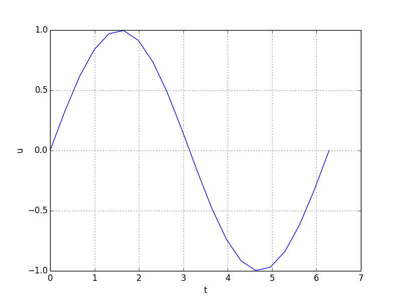
This seemingly simple algorithm actually accomplishes something quite complex with a few lines. The magic is in lines 32-24. When an algorithms sets the CONTINUE_EXECUTING() key, the pipeline will execute again both the RequestUpdateExtent() and RequestData() passes. So let’s trace what this algorithm does:
- In RequestInformation(), it initializes a few data members including UpdateTimeIndex.
- In RequestUpdateExtent(), it sets the update time value to the first time step (because UpdateTimeIndex == 0).
- Upstream pipeline executes.
- In RequestData(), it stores the u value of the first point in the ValueOverTime array as the first value (using UpdateTimeIndex as the index).
- Because we didn’t reach the last time step, it increments UpdateTimeIndex and sets CONTINUE_EXECUTING().
- The pipeline re-executes the filter starting at 2. But this time UpdateTimeIndex is 1 so the upstream will produce the 2nd time step.
This will continue until UpdateTimeIndex == len(self.TimeValues) – 1. Once the streaming is done, the filter adds its cached value to its output as an array.
There you go, streaming in a nutshell. This can be used to do lots of useful things such as computing temporal mean, min, max, standard deviation etc etc. It can be also used to do more sophisticated things such as a particle advection. I will cover that in my next blog. If you are up to the challenge, here are a few tips:
- Start with a set of seed points (say a line parallel to the y axis),
- Stream timesteps 2 at a time,
- For each pair of time steps, calculate the mean velocity,
- Calculate the next set of points as pnext = pprev + vel * dt,
- You can compute the vel at each point by using the probe filter.
This should give you a very basic first order particle integrator. The solution in the next blog…
Note: A more thorough description of the temporal streaming in VTK can be found in this paper.