The VTK Parallel Statistics Module

The addition of a parallel, scalable statistics module to VTK was motivated by the Titan Informatics Toolkit, a collaborative effort between Sandia National Laboratories and Kitware. This effort significantly expanded VTK to support the ingestion, processing, and display of informatics data. By leveraging the VTK data and execution models, Titan provides a flexible, component based, pipeline architecture for the integration and deployment of algorithms in the fields of intelligence, semantic graphing, and information analysis.
In 2008, the parallel statistical engineers were integrated into VTK, and the module has continued to grow as new engines developed in the context of the “Network Grand Challenge” LDRD project at Sandia, and under a DOE/ASCR program to conduct broad research in the topological and statistical analysis of petascale data. As a result, a number of univariate, bivariate, and multivariate statistical engines have been implemented in VTK.
In this article we summarize the general design of these classes, describe the specifics of each, and conclude by mentioning an ongoing collaboration in the field of computational combustion science that is making use of the most recent addition to the VTK parallel statistics module.
Variables & Operations
Each of the engines operates upon data stored in one-or-more vtkTable instances, where the first table contains “observations” and further tables represent statistical models. The statistical analysis algorithms are partitioned into four disjoint operations in order to meet two overlapping but not exactly congruent design requirements: 1) the algorithms should match typical statistical data analysis workflows; and 2) the algorithms should lend themselves to scalable parallel implementations. The four operations include the following: learn a model from observations; derive statistics from a model; assess observations with a model, and test a hypothesis.
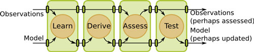
Figure 1: The 4 operations of statistical analysis and their interactions with input observations and models. When an operation is not requested, it is eliminated by connecting input to output ports.
These operations, once executed, occur in order as shown in Figure 1. However, it is also possible to execute only a subset of these; for example, when it is desired to have previously computed models, or models constructed with expert
knowledge, be used in conjunction with existing data.
These operations, performed on a request comprising a set of columns of the input observations table, are detailed as follows:
Learn: Calculate a “raw” statistical model from an input dataset. By “raw,” we mean the minimal representation of the desired model, which contains only primary statistics. For example, in the case of descriptive statistics: sample size, minimum, maximum, mean, and centered M_2, M_3 and M_4 aggregates1.
Derive: Calculate a “full” statistical model from a raw model. By “full,” we mean the complete representation of the desired model, which contains both primary and derived statistics. For example, in the case of descriptive statistics, the following derived statistics are calculated from the raw model: unbiased variance estimator, standard deviation, and two estimators for both skewness and kurtosis.
Assess: Given a statistical model — from the same or another dataset — mark each datum of a given dataset.
Test: Given a set of observations and a statistical model, perform statistical hypothesis testing.
Algorithms
The following algorithms are currently available in the VTK parallel statistics module. We are not discussing the Test operation, which is still considered experimental and not yet available for all engines.
Univariate Statistics
Descriptive Statistics:
Learn: Calculate minimum, maximum, mean, and centered M_2, M_3 and M_4 aggregates.
Derive: Calculate unbiased variance estimator, standard deviation, skewness (1_2 and G_1 estimators), kurtosis (g_2 and G_2 estimators).
Assess: Mark with relative deviations (one-dimensional Mahalanobis distance).
Order Statistics:
Learn: Calculate histogram.
Derive: Calculate arbitrary quantiles, such as “5-point” statistics (quantiles) for box plots, deciles, percentiles, etc.
Assess: Mark with quantile index.
Auto-Correlative Statistics:
Learn: Calculate minimum, maximum, mean, and centered M_2 aggregates for a variable with respect to itself for a set of specified time lags (i.e., time steps between datasets of equal cardinality that are assumed to represent the same variable distributed in space).
Derive: Calculate unbiased auto-covariance matrix estimator and its determinant, Pearson auto-correlation coefficient, linear regressions (both ways), and fast Fourier transform of the auto-correlation function, again for a set of specified time lags.
Assess: Mark this with the squared two-dimensional Mahalanobis distance.
Bivariate Statistics
Correlative Statistics:
Learn: Calculate the minima, maxima, means, and centered M_2 aggregates.
Derive: Calculate unbiased variance and covariance estimators, Pearson correlation coefficient, and linear regressions (both ways).
Assess: Mark with the squared two-dimensional Mahalanobis distance.
Contingency Statistics:
Learn: Calculate contingency table.
Derive: Calculate joint, conditional, and marginal probabilities, as well as information entropies.
Assess: Mark with joint and conditional PDF values, as well as pointwise mutual informations.
Multivariate Statistics
These filters all accept requests containing n_i variables upon which simultaneous statistics should be computed.
Multi-Correlative Statistics:
Learn: Calculate the means and pairwise centered M_2 aggregates.
Derive: Calculate the upper triangular portion of the symmetric n_i*n_i covariance matrix and its (lower) Cholesky decomposition.
Assess: Mark with the squared multi-dimensional Mahalanobis distance.
PCA Statistics:
Learn: Identical to the multi-correlative filter.
Derive: Everything the multi-correlative filter provides, plus the n_i eigenvalues and eigenvectors of the covariance matrix.
Assess: Perform a change of basis to the principal components (eigenvectors), optionally projecting to the first m_i components, where m_i < n_i is either a user-specified value or is determined by the fraction of maximal eigenvalues whose sum is above a user-specified threshold. This results in m_i additional columns of data for each request R_i.
K-Means Statistics:
Learn: Compute optimized set(s) of cluster centers from initial set(s) of cluster centers. In the default case, the initial set comprises the first K observations. However, the user can specify one-or-more sets of cluster centers (with possibly differing numbers of clusters in each set) via an optional input table, in which case an optimized set of cluster centers is computed for each of the input sets.
Derive: Calculate the global and local rankings amongst the sets of clusters computed in the learn operation. The global ranking is the determined by the error amongst all new cluster centers, while the local rankings are computed amongst clusters sets with the same number of clusters. The total error is also reported.
Assess: Mark with closest cluster id and associated distance for each set of cluster centers.
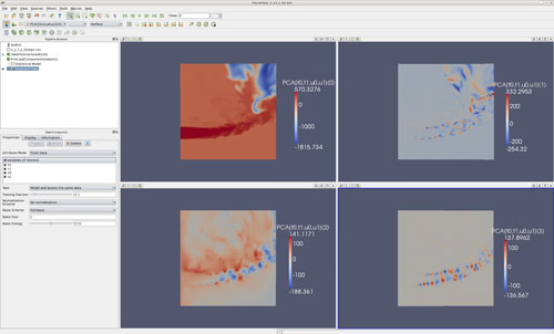
Figure 2: Several of the VTK parallel statistics engines are integrated into ParaView. Example using PCA on four dataset attributes
An example of the statistical engines within ParaView is shown in Figure 2. In this example, a PCA analysis is performed on a quadruple of variables of interest in a 2D flame simulation, whereby the statistical model is calculated (learn and derive operations) on a randomly-sampled subset of 1/10-th of the entire dataset, after which all points in the dataset are marked with their respective relation deviations from this model.
Input and Output Ports
The statistics algorithms have by default three input ports and three output ports as follows:
Input Port 0: This port is identified as vtkStatisticsAlgorithm::INPUT_DATA and is used for learn data.
Input Port 1: This port is identified as vtkStatisticsAlgorithm::LEARN_PARAMETERS and is used for learn parameters (e.g., initial cluster centers for k-means clustering, time lags for auto-correlation, etc.).
Input Port 2: This port is identified as vtkStatisticsAlgorithm::INPUT_MODEL and is used for a priori models.
Output Port 0: This port is identified as vtkStatisticsAlgorithm::OUTPUT_DATA and it mirrors the input data and optional assessment columns.
Output Port 1: This port is identified as vtkStatisticsAlgorithm::OUTPUT_MODEL and contains any generated model.
Output Port 2: This port is identified as vtkStatisticsAlgorithm::OUTPUT_TEST and is currently experimental and not used by all statistics algorithms. Please note that in earlier implementations it was called vtkStatisticsAlgorithm::ASSESSMENT, a key which has since been deprecated.
All input and output ports are all of type vtkTable, with the exception of both input and output ports 1 which are of type vtkMultiBlockDataSet. Note that this is an update from earlier implementations of these filters where it was also possible for ports 1 to be of type vtkTable, however that is no longer the case.
Parallel Statistics Classes
The purpose of building a full statistical model in two separate operations is two-fold: database normalization (resulting from the fact that there is no redundancy in the primary model) and parallel computational efficiency. As a result, in our approach, inter-processor communication and updates are performed only for primary statistics.
The calculations for obtaining derived statistics from primary statistics are typically fast and simple and need only be calculated once, without communication, upon completion of all parallel updates of primary variables. Data to be assessed is assumed to be distributed in parallel across all processes participating in the computation; thus, no communication is required as each process assesses its own resident data.
Therefore, in the parallel versions of the statistical engines, inter-processor communication is required only for the Learn operation, while both Derive and Assess are executed in an embarrassingly parallel fashion due to data parallelism. This design is consistent with the methodology used to enable parallelism within VTK, most notably in ParaView.
The following 8 parallel statistics engines are implemented and available in the parallel statistics module of VTK: vtkPAutoCorrelativeStatistics; vtkPDescriptiveStatistics; vtkPOrderStatistics; vtkPCorrelativeStatistics; vtkPContingencyStatistics; vtkPMultiCorrelativeStatistics; vtkPPCAStatistics; vtkPKMeansStatistics.
Each of these parallel algorithms is implemented as a subclass of the respective serial version of the algorithm and contains a vtkMultiProcessController for handling inter-processor communication.
Within each of the parallel statistics classes, the Learn operation is the only operation whose behavior is changed (by reimplementing its virtual method or by reimplementing virtual methods that are called by the Learn operation). The Dervie and Assess operations remain unchanged due to their inherent data parallelism. The Learn operation of the parallel algorithms performs two primary tasks:
1. Calculate statistics on local data by executing the Learn code of the superclass.
2. If parallel updates are needed (i.e. the number of processes is greater than one), perform the necessary data gathering and aggregation of local statistics into global statistics.
The descriptive, correlative, auto-correlative and multi-correlative statistics algorithms perform the aggregation necessary for the statistics which they are computing using the arbitrary-order update and covariance update formulas presented in [1]. Since the PCA statistics class derives from the multi-correlative statistics algorithm and inherits its Learn operation, a static method is defined within the parallel multi-correlative statistics algorithm to gather all necessary statistics. As we have demonstrated in [2], all those parallel classes exhibit optimal parallel speed-up properties.
Similarly, the contingency statistics class derives from the bivariate statistics class and implements its own aggregation mechanism for the Learn operation. However, unlike the other statistics algorithms which rely on statistical moments (descriptive, correlative, auto-correlative, multi-correlative, PCA, and K-means), this aggregation operation is, in general, not embarrassingly parallel; therefore, optimal parallel scale-up is not observed when this class is not used outside of its intended domain of applicability. The same is the case for the order statistics, since the parallel update of a histogram involves more than negligibly small amounts of data as compared to the overall dataset size.
Usage
It is fairly easy to use the serial statistics classes of VTK; it is not much harder to use their parallel versions. All that is required is a parallel build of VTK and a version of MPI installed on your system.
Listing 1: A subroutine that should be run in parallel for calculating auto-correlative statistics.
void Foo( vtkMultiProcessController* controller, void* arg )
{
// Use the specified controller on all parallel
filters by default:
vtkMultiProcessController::SetGlobalController( controller );
// Assume the input dataset is passed to us:
vtkTable* inputData = static_cast<vtkTable*>( arg );
// Create parallel auto-correlative statistics class
vtkPAutoCorrelativeStatistics* pas = vtkPAutoCorrelativeStatistics::New();
// Set input data port
pas->SetInput( 0, inputData );
// Select all columns in inputData
for ( int c = 0; c < inputData->GetNumberOfColumns(); ++ c )
{
pas->AddColumn( inputData->GetColumnName[c] );
}
// Set spatial cardinality
pas->SetSliceCardinality( nVals );
// Set parameters for autocorrelation of whole dataset with respect to itself
pas->SetInputData( vtkStatisticsAlgorithm::LEARN_PARAMETERS, paramTable );
// Calculate statistics with Learn and Derive operations only
pas->SetLearnOption( true );
pas->SetDeriveOption( true );
pas->SetAssessOption( false );
pas->SetTest( false );
pas->Update();
}
Listing 1 demonstrates how to calculate auto-correlative statistics in parallel on each column of an input set inData, which is a pointer to a vtkTable instance with an associated set of input parameters and no subsequent data assessment.
It is assumed that this input data type is of numeric type (i.e. double), with the following storage convention: each time-step corresponds to a block of data of the same size denoted nVals above. Each block is often referred to as a time-slab. As a result, there are as many data points for each variable as there are time steps, times the slab size nVals.
A parameter table paramTable contains the list of time lags of interest; i.e., those time steps for which the auto-correlation must be computed with respect to the initial time step (the first slab in the dataset). In particular, if this parameter table contains only one entry with value ~0, then the auto-correlation of the entire dataset against itself will be calculated, which will lead to a covariance matrix with all coefficients equal to the variance of the variable, and the auto-correlation coefficient will be equal to 1.
For univariate statistics algorithms calling AddColumn() for each column of interest sufficient — each request can by definition only reference a single column and so the filter automatically turns each column of interest into a separate request. However, this is not sufficient for multivariate filters as each request might have a different number of columns of interest. In this case, requests for columns of interest are specified by calling SetColumnStatus() multiple times to identify the variables to be used, followed by a call to RequestSelectedColumns().
The examples thus far assume that a vtkMPIcommunicator was previously prepared within the parallel environment used to execute the parallel auto-correlative statistics engine. It is outside the scope of this article to discuss I/O issues, and in particular how a vtkTable instance can be created and filled with the values of the variables of interest (see the online documentation of VTK or its user manual for details). However, we include a small amount of code to prepare a parallel controller.
Listing 2: A snippet of code to show how to execute a subroutine (Foo()) in parallel. In reality, inData would be prepared in parallel by Foo() but is assumed to be pre-populated here to simplify the example.
vtkTable* inputData;
vtkMPIController* controller = vtkMPIController::New();
controller->Initialize( &argc, &argv );
// Execute the function named Foo on all processes
controller->SetSingleMethod( Foo, &inputData );
controller->SingleMethodExecute();
// Clean up
controller->Finalize();
controller->Delete();
In the code example from Listing 1, the vtkMultiProcessController object passed to Foo() is used to determine the set of processes (which may be a subset of a larger job) among which input data is distributed. VTK uses subroutines of this form to execute code across many processes.
In order to prepare a parallel controller to execute Foo() in parallel with MPI, one must first (e.g. in the main routine) create a vtkMPIController instance and pass it the address of Foo(), as shown in Listing 2. Note that, when using MPI, the number of processes is determined by the external program which launches the application.
An Application to Computational Combustion
As an example of the application of the VTK parallel statistic module, we discuss an ongoing effort in collaboration with Dr. Jacqueline Chen’s research group at Sandia National Laboratories, for the analysis of Direct Numerical Simulation (DNS) of reactive flows using the auto-correlation engine that was recently added to the statistics module.
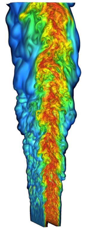 Figure 3: A lifted ethylene jet flame generated from a direct numerical simulation
(image courtesy of Hongfeng Yu and Jacqueline Chen).
Auto-correlation is the cross-correlation of a signal with itself, providing a measure of the similarity between observations as a function of the time separation between them. It is typically used to discover underlying repeating patterns in the presence of noise. Within the context of the analysis of DNS computations, it is the prevalent method used by the combustion community to measure the turbulence spectrum and the turbulence length scales.
In an Eulerian framework, the turbulent eddies in a homogeneous turbulent flow can be perceived as being transported across a point of observation at a rate equal to the mean velocity. The integral time scale, which is computed as the time integration of the autocorrelation function, can be used to deduce the integral length scale through a space-time transformation. The Fourier transform of the autocorrelation function yields the turbulent frequency spectrum, whose integer is the mean square of the velocity fluctuation.
The ongoing effort aims at providing in-situ or in-transit auto-correlation analysis to flame simulations as illustrated in Figure 3 in particular to measure turbulence spectrum and length scales. For more detail about the type of simulations involved and the approach used for large scale data analysis in this context, please refer to [3].
Acknowledgements
This work was initially supported by the laboratory-directed research & development (LDRD) “Network Grand Challenge” project, and afterwards by the “Mathematical Analysis of Petascale Data” project of the Advanced Scientific Computing Research (ASCR) office of the U.S. DOE. The authors would like to express their gratitude to Sandy Landsberg, ASCR project manager, for her continued support for this work, and to David Thompson (Sandia/Kitware) for his early contributions to this project.
Sandia National Laboratories is a multi-program laboratory managed and operated by Sandia Corporation, a wholly owned subsidiary of Lockheed Martin Corporation, for the U.S. Department of Energy’s National Nuclear Security Administration under contract DE-AC04-94AL85000.
 Philippe Pébay is Technical Expert in Visualization and HPC at Kitware SAS, the European subsidiary of the Kitware group. Pébay is currently one of the most active developers of VTK, an open-source, freely available software system for 3D computer graphics, image processing, visualization, and data analysis. He is in particular the main architect of the statistical analysis module of VTK and ParaView.
 Janine Bennett is a Principal Member of the Technical Staff in the Scalable Modeling and Analysis Systems Department at Sandia National Laboratories. Janine’s research focuses on data analysis challenges in extreme-scale HPC environments and her interests include feature segmentation, scalable statistics algorithms, computational geometry, combinatorial topology, emerging programming and execution models, and analysis of uncertain data.
References:
- P. Pébay, Formulas for robust, one-pass parallel computation of covariances and arbitrary-order statistical moments. Sandia Report SAND2008-6212, Sandia National Laboratories, September 2008.]
- P. Pébay, D. Thompson, J. Bennett, and A. Mascarenhas. Design and performance of a scalable, parallel statistics toolkit. In Proc. 25th IEEE International Parallel & Distributed Processing Symposium, 12th International Workshop on Parallel and Distributed Scientific and Engineering Computing. Anchorage, AK, U.S.A., May 2011.
- J. Bennett et al., “Combining in-situ and in-transit processing to enable extreme-scale scientific analysis”, Proc. Supercomputing 2012 International Conference for High Performance Computing, Networking, Storage and Analysis. Salt Lake City, UT, U.S.A., November 2012]