
Visualization & Analysis of AMR Datasets

Multiphysics simulations of complex phenomena exhibiting large length and time scales, such as astrophysics, have been greatly facilitated by the AMR approach. By discretizing the computational domain with multiple, overlapping, uniform grids of varying resolution, high-fidelity accuracy can be attained in regions of interest where high-resolution, uniform grids are employed. Lower-resolution is used where the solution is not changing to reduce memory and storage requirements; however, the nested grid structure poses new challenges for the visualization and analysis of such datasets. Specifically, visualization algorithms need to process a dynamic hierarchy of grids that change at each time-step and properly handle the overlapping regions and inter-level grid interfaces. At the same time, the size generated from typical simulations can be prohibitively large, necessitating the development of new visualization approaches that enable scientists and engineers to analyze their data. The enabling technology for visualization and analysis at such large scales is query-driven visualization[3] and is the primary and ongoing goal of this work.
The basic idea of query-driven visualization is to selectively load data within a user-supplied region of interest (ROI). It is rooted in the observation that most of the insights are derived from only a small subset of the dataset [4,5]. For example, the user may request to visualize the data at a specific level of resolution, or just a slice of the data. To this end, we have developed an extensible and uniform software framework for AMR datasets that supports loading of data on-demand, as well as handling of particles. Further, we have implemented a slice filter that operates directly on AMR data and produces 2-D AMR slices that enables the inspection of volumetric data in varying resolutions. Lastly, we have developed an AMR dual-grid extraction filter that normalizes the representation of cell-centered AMR data to an unstructured grid and allows the use of existing contouring algorithms (i.e., Marching Cubes (MC)) for iso-surface extraction without further modification. The remainder of this article discusses the aforementioned developments in more detail.
AMR Data Structures
The algorithms and operations for query-driven visualization are best described by first presenting the underlying VTK AMR data-strucutres. Although there are several variations of AMR, our implementation focuses on Structured AMR datasets where the solution is stored at the cell centers. In particular, the algorithms and operations described herein focus on the Berger-Collela AMR scheme [1,2], which imposes the following structure:
- All grids are Cartesian.
- Grids at the same level do not overlap.
- The refinement ratios, RL, between adjacent levels are integer (typically 2 or 4) and uniform within the same level.
- Grid cells are never partially refined; i.e., each cell is refined to four quads in 2D or eight hexahedra in 3D.
A sample 2-D AMR dataset with two levels and a refinement ratio, RL=4, is shown in Figure 1. Note that the low-resolution cells that are covered by high-resolution grids, shaded by green and red wireframe colors, are hidden.
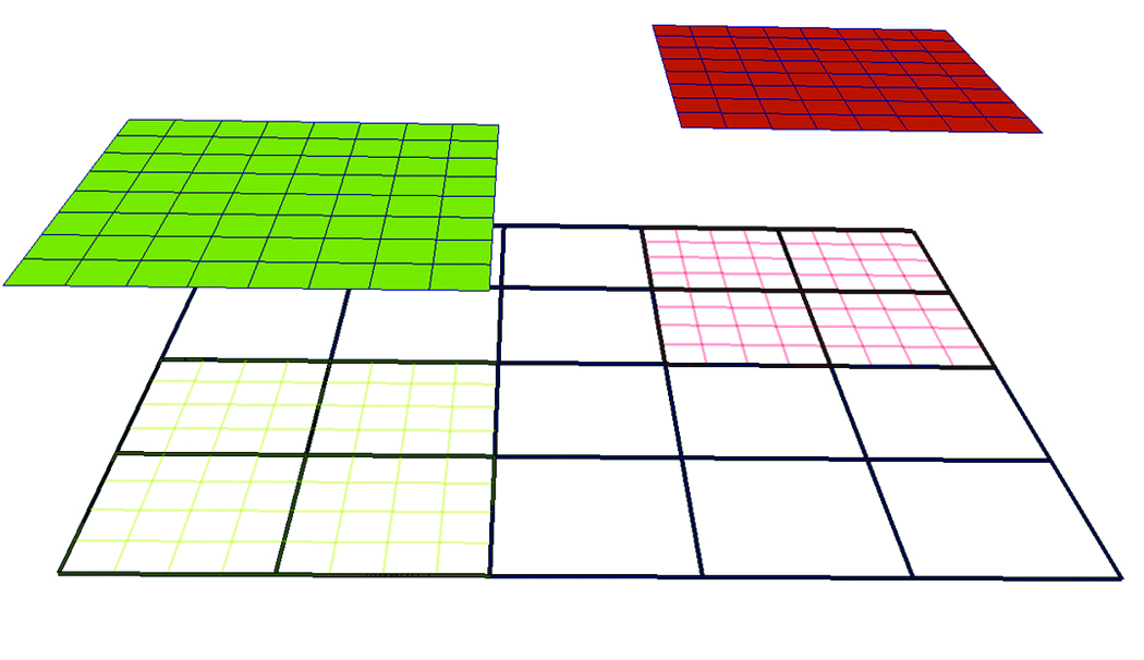
Figure 1. Sample 2D AMR Dataset with two levels and refinement ratio, RL=4. The root level (L0) consists of a single grid shown in black wireframe while the next level (L1) consists of two grids, depicted in green wireframe and red wireframe respectively. The
two grids at L1 are projected from the root level to illustrate that the cells underneath are “hidden.”
In VTK, the collection of AMR grids is stored in a vtkHierarchicalBoxDataSet data-structure. Each grid, G(Li,k), is represented by a vtkUniformGrid data structure where the unique key pair (Li,k) denotes the corresponding level (Li) and the grid index within the level (k) with respect to the underlying hierarchical structure. An array historically known as IBLANK, stored as a cell attribute in
vtkUniformGrid, denotes whether a cell is hidden or not. The blanking array is subsequently used by the mapper to hide lower resolution cells accordingly when visualizing the dataset.
However, the size of the data generated for typical simulations prohibits loading the entire dataset in memory. Even in a parallel, distributed memory environment, loading the entire dataset in memory is not a practical solution for most interactive visualization tasks on AMR datasets. Most of the time, scientists and engineers interact with their datasets by either performing queries that concentrate on a sub-region (e.g., a slice of the data at a given offset), or perform operations that can operate in a streaming fashion (e.g., computing derivatives or other derived attributes). To enable the execution of such queries without loading
the entire dataset in memory, metadata information is employed. The metadata stores a minimal set of geometric information for each grid in the AMR hierarchy. Specifically, the AMR metadata, B(Li,k), corresponding to the grid G(Li,k), is represented using a vtkAMRBox object and it consists of the following information:
- N={Nx, Ny, Nz} — the cell dimensions of the grid (since the data is cell-centered)
- The grid spacing at level L, hL={hx,hy,hz}
- The grid level Li and grid index k
- The global dataset origin, X=(X0, Y0, Z0), i.e., the minimum origin from all grids in level L0 and
- The LoCorner and HiCorner, which describe the low and high corners of the rectangular region covered by the corresponding grid in a virtual integer lattice with the same spacing (h) that covers the entire domain.
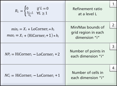
Table 1. Common relationships to derive grid information from AMR box metadata.
Given the metadata information stored in the AMR box of each grid, the refinement ratio at each level can be easily computed using relationship (1) from Table 1. Further, the cartesian bounds the corresponding grid covers and the number of points and cells is also available (see relationships 2-4 in Table 1). Notably, geometric queries such as determining which cell contains a given point, or if a grid intersects a user-supplied slice plane, can be answered using just the metadata. With this approach, data that satisfies a given query can be loaded into memory for analysis and visualization more efficiently through inspection of the metadata.
Query-Driven AMR Visualization Framework
The core functionality for query-driven visualization is provided by employing a lazy-loading design pattern, which defers loading the data until it is requested. This imposes slightly different requirements in the design and implementation of readers and filters for query-driven visualization. First, AMR readers must implement functionality for (a) loading the metadata given an input file and (b) for accepting data requests from downstream filters and/or interactively by the user. Second, filters must implement functionality for sending data requests upstream to the reader according to user-supplied input. To make this concept more concrete, consider slicing an AMR dataset at a low resolution and inspecting the volume as a simple example. Typically, once the region of interest is identified, a higher resolution slice would be required for further analysis. Allowing users to increase the resolution on a slice triggers an upstream request to the reader to load the blocks to the prescribed level of resolution that intersect the given planar slice. Efforts are ongoing in enhancing the VTK pipeline to better support this type of demand-driven operation within ParaView. In this section, we present preliminary work towards that goal, specifically targeting AMR datasets.
Query-Driven AMR Readers
Typical AMR codes, such as Enzo [6,7] and FLASH [8], are hybrid codes that combine both the fluid quantities (e.g., density, velocity, etc) defined on the AMR grid hierarchy with particle quantities (e.g., mass, position, etc.) in a single set of coupled governing equations. Hence, the capability to visualize both the particles and AMR grid datatypes is crucial in the analysis of such datasets. Two separate readers are implemented in our framework to address the separate queries required for each datatype (AMR grids and particles) respectively. A schematic class diagram of the readers implemented is depicted in Figure 2.
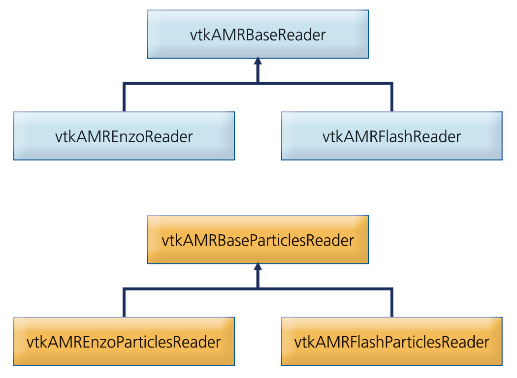
Figure 2. Schematic class diagram of AMR and particle data readers.
The abstract base classes implement common functionality to all AMR and particle readers respectively. Specifically, they define a common API, implement common UI components, and implement assignment of blocks to different processes when running in a distributed environment. In this approach, the user interface of all concrete AMR and particle readers is consistent and a set of common operations is guaranteed. In the present implementation, the framework has native support for Enzo and Flash datasets. Native support for other AMR datasets, such as RAMSES and Orion, is also projected in the future.
Typical operations the AMR reader provides for fluid data analysis include the ability to specify the maximum level of resolution and select which attributes to load. This functionality is extremely useful when loading large-scale datasets since most of the time loading the entire dataset in memory is not feasible. By loading just a couple of low resolution levels, users gain insight as to where potential regions of interest are and extract those regions for further analysis. Figure 3 (a) depicts the reader panel accessible from ParaView that illustrates the user controls currently enabled; namely, the ability to select a maximum level of resolution and which attributes to load. Figure 3 (b) shows the resulting surface mesh when prescribing a maximum resolution of seven.
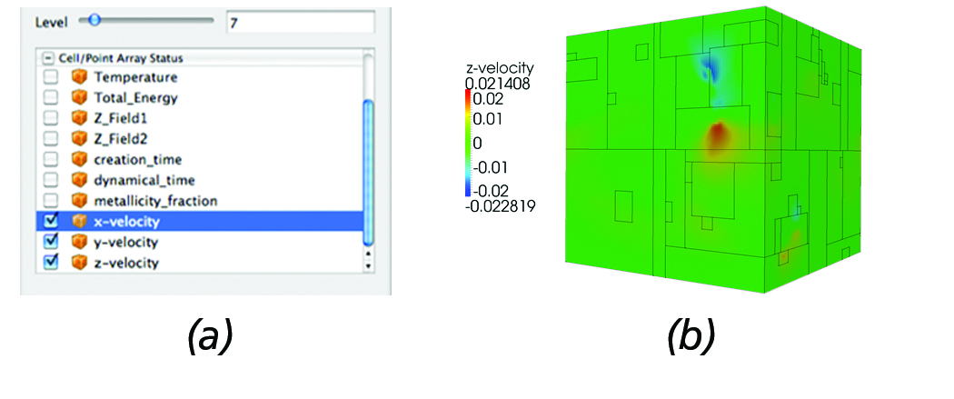
Figure 3. AMR Reader: (a) The reader panel that provides functionality for selectively loading cell/point data and controlling the
maximum desired level of resolution. (b) Surface mesh of the Enzo AMR Red-Shift dataset with the outline of each block overlayed.
Similar functionality is also enabled for the particle readers. Figure 4 (a) depicts the particle reader panel controls and (b) shows the resulting particle dataset. As with the AMR reader, the ability to select which attributes to load is enabled. Further, using a frequency parameter, particles can be subsampled; for example: in this case, the reader will load every other five particles, an operation that is commonly employed when analyzing particle simulations. In addition, particles can be filtered based on location or by particle type (e.g., in the case of Enzo datasets, Dark Matter, Start, or Tracer particles can easily hidden/shown).
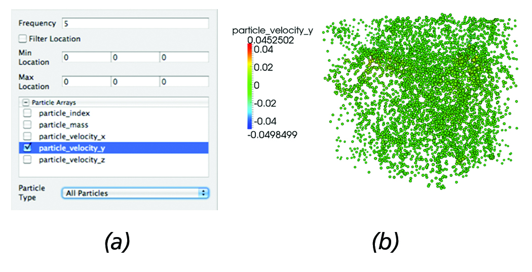
Figure 4. Particles Reader: (a) Reader panel that provides functionality for sub-sampling; e.g., in this case, every five particles are loaded, selective loading of particle arrays, filtering particles within a bounding box defined by its min and max coordinates, as
well as filtering particles by type (e.g., in the case of Enzo datasets filtering by Dark Matter, Star or Tracer particles). (b) Corresponding particle dataset represented using point-sprites where each particle radius is proportional to the y-velocity.
AMR Slice Operator
One of the most fundamental yet effective approaches for analyzing 3D AMR datasets is extraction of axis-aligned AMR slices through the dataset. Benefits to this approach include the simple calculation of which blocks to load, and the ability to exploit the multi-resolution, hierarchical data-structure within the slice. The AMR Slice operator is implemented in vtkAMRSliceFilter, a concrete implementation of the vtkHierarchicalBoxDataSetAlgorithm. It accepts as input a 3D AMR dataset, and produces a 2D AMR dataset at a user-supplied offset.
Given an offset (dx) and and axis-aligned plane (Pi= {XY,XZ,YZ}), construction of the 2D AMR dataset is achieved in the following steps:
- Construct the cutplane, P, positioned dx from the global dataset origin provided by the AMR metadata (recall section 2).
- Given the bounds of each block from the metadata, determine which blocks intersect with the cutplane, P.
- For each block, create a 2D vtkUniformGrid instance along the plane P.
- Copy the solution from the 3D blocks to the corresponding 2D cells (direct injection).
Figure 5(b) shows the output generated by the AMR slice filter for the parameters set in Figure 5(a) as a simple example demonstrating the present functionality. It should be noted that in the present implementation, by increasing the resolution (level), upstream requests for higher resolution blocks are sent to the reader.
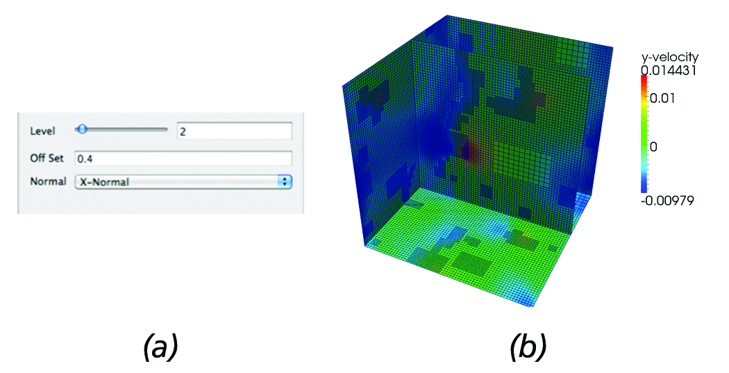
Figure 5. AMR Slice: (a) Slice filter panel controls that allow users to set the offset of the slice and request a higher resolution data to be loaded. (b) Resulting 2D AMR slice data @dx=0.4 from the global dataset origin overlayed on the surface mesh of the
computational domain.
Another commonly employed task used in the analysis of AMR simulations involves over-plotting the particles within a user-supplied distance from the slice. In the given framework, this is easily achieved by using the slice filter in conjuction with the particles reader and filtering out particles within the region of interest. This use case is illustrated in Figure 6. First, the slice is created and positioned at the region of interest. Then, all particles within [0.2, 0.4] along the x-axis and desired particle data are loaded, see Figure 6(a).
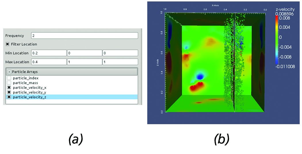
Figure 6. Overplotting Particles on a slice. (a) AMR particles reader panel configuration. (b) Resulting slice with particles overlayed
withing the prescribed region.
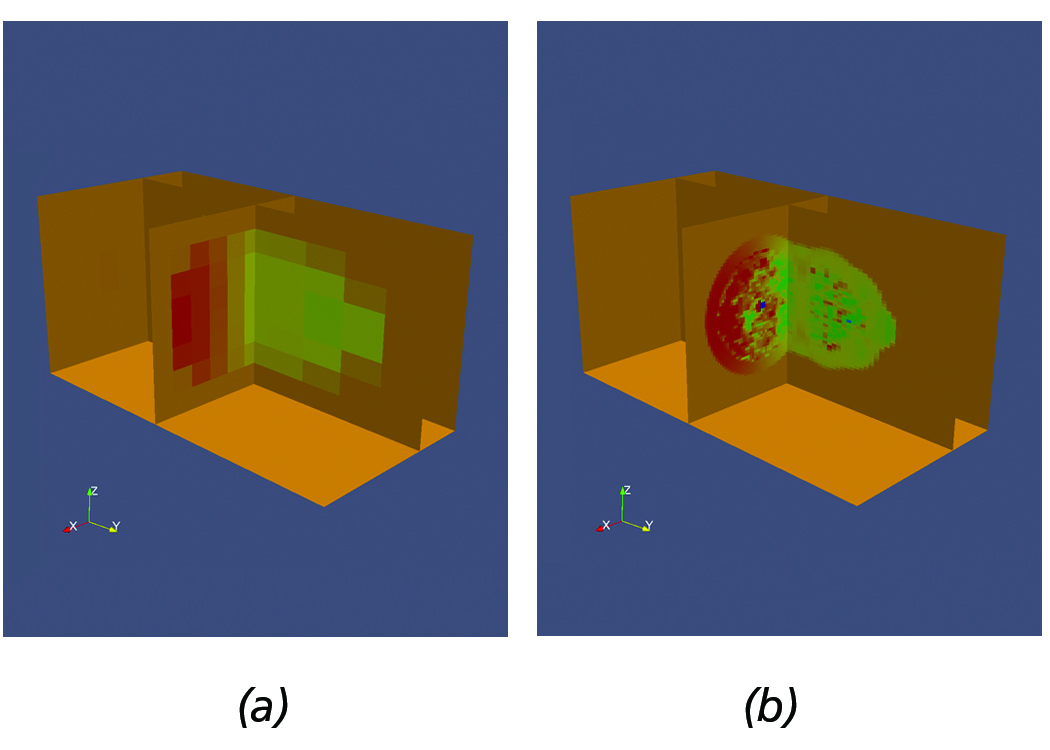
Figure 7. Sample Flash dataset demonstrating the use of multi-resolution slicing. (a) Low resolution. (b) Increased resolution.
Slicing AMR datasets is a very powerful technique, especially when analyzing very large datasets. Scientists typically initially
load the data at a low-resolution, create a slice, and sweep within the volume until they find regions of interest.
Once a region of interest is identified, scientists can increase the resolution to gain further insight into the physical phenomena
and subsequently use other filters to perform other quantitative analysis, e.g., plots etc. within the slice. For example, Figure 7(a) shows a sample Flash dataset with slices positioned within a region of interest, acquired by sweeping the volume of the AMR dataset. Next, Figure 7(b) shows the slices after requesting higher resolution data to be loaded.
Dual-Based Iso-Surface Extraction of AMR Datasets
Iso-surface extraction is a fundamental technique employed for qualitative analysis of scalar fields. However, without proper handling of AMR data, the use of commonly employed techniques, such as the Marching Cubes (MC) [9], is complicated by discontinuities at the inter-level interfaces.
To address this issue, we have implemented a vtkAMRDualExtractionFilter, which constructs a dual-mesh (i.e., the mesh constructed by connecting the cell-centers) over the computational domain that can be subsequently used for extracting the iso-surfaces by the MC approach.
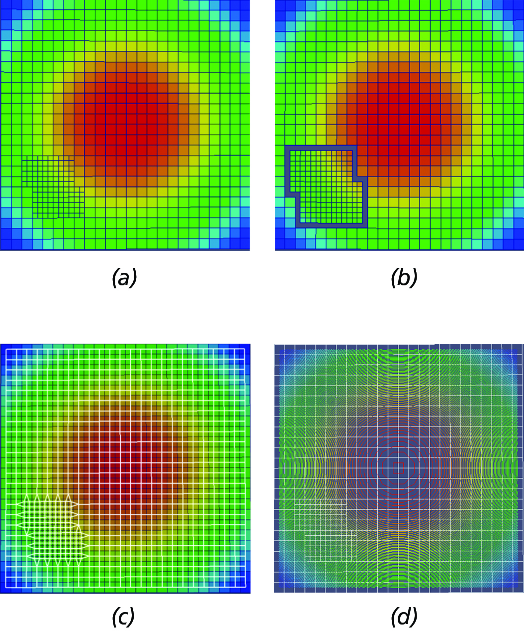
Figure 8. Primary steps of dual-based, iso-surface extraction algorithm. (a) Initial AMR grid hierarchy configuration. (b) AMR
dual with gaps at the inter-level interfaces. (c) Stiched dual mesh (in white wireframe) overlayed by the original grid. (d) Contour
constructed by the MC algorithm using the dual-mesh overlayed by the original AMR grid configuration shown in white wireframe.
For a schematic depiction of the primary steps of the dual-based, iso-surface extaction approach implemented in this work, see Figure 8. At a high-level, the main steps of the algorithm are the following:
- Extract one layer of ghost-cells and transfer (direct injection) the solution from the adjacent cells of lower or equal resolution.
- Process each block separately and generate the dual mesh, M. Note: this approach introduces gaps where there is a level difference (See Figure 8(b)).
- Stitch the gaps by moving the nodes of the dual mesh (M) to the centroid of the adjacent lower resolution cells, i.e., Figure 8(c).
- Pass the modified dual mesh to the MC for contouring, i.e., see Figure 8(d).
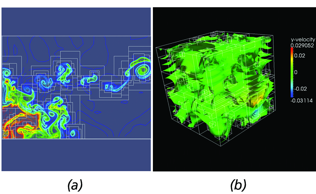
Figure 9. Dual-based contours from complex AMR datasets. (a) Contours from implosion AMR dataset. (b) 3-D contours from Red-Shift AMR dataset.
Although the current implementation is not yet at a production state, our approach has been successfully employed with complex AMR datasets, such as the Implosion Enzo AMR sample dataset shown in Figure 9(a) and the 3D Redshift AMR dataset depicted in Figure 9(b).
Concluding Remarks
Current progress towards the development of a query-driven visualization framework targeting large-scale AMR datasets is presented with preliminary results. Ongoing efforts focus on further exploiting the VTK pipeline to better suit query-driven operations; implementation of new operators and more readers, such as RAMSES and Orion; integration with domain specific toolkits, such as yt [10]; and investigating approaches for query-driven volume rendering.
Acknowledgements
The work presented in this article is funded by DOE under Phase II SBIR Contract No. DE-FG02-09ER85461. The authors would like to thank Matt Turk from the Department of Astronomy at Columbia University and Paul Sutter from the University of Illinois at Urbana-Champaign for their insightful discussions and for providing astrophysical simulation datasets. Further, the authors would like to thank Utkarsh Ayachit, Robert Maynard, Sebastien Jourdain, and Dave DeMarle for helpful technical discussions.
References
[1] M. J. Berger and P. Colella. Local Adaptive Mesh Refinement for Shock Hydrodynamics. Journal of Computational Physics,
82:64-84, 1989.
[2] K. Stockinger, H. Hagen, K. Wu and E. W. Bethel. Query-Driven Visualization of Large Datasets. In Proceedings of IEEE
Visualization, 167-174, 2005.
[3] J. Becla and D. L. Wang. Lessons Learned from Managing a Petabyte. In Proceedings of Innovative Data Systems Research,
70-83, 2005.
[4] J. Gray, D. T. Liu, M. A. Nieto-Santisteban, A. S. Szalay, D. J. DeWitt and G. Heber. Scientific Data Management in the Coming
Decade. SIGMOD Record, 34(4):34-41, 2005.
[5] G. L. Bryan and M. L. Norman. A Hybrid AMR Application for Cosmology and Astrophysics. ArXiv Astrophysics e-prints.
http://arxiv.org/abs/astro-ph/9710187
[6] J. O. Burns, S W. Skillman and B. W. O’Shea. Galaxy Clusters at the Edge: Temperature, Entropy, and Gas Dynamics Near the
Virial Radius. The Astrophysics Journal, 721, 1105, 2010.
[7] B. Fryxell, K. Olson, P. Ricker, F. X. Timmes, M. Zingale, D. Q. Lamp, P. MacNeice, R. Rosner, J. W. Trunan and H. Tufo.
FLASH: An Adaptive Mesh Hydrodynamics Code for Modeling Astrophysical Thermonuclear Flashes. The Astrophysical Journal
Supplement Series, 131:273-334, 2000.
[8] W. E. Lorensen and H. E. Cline. Marching Cubes: A High Resolution 3D Surface Construction Algorithm. Computer Graphics
(SIGGRAPH ’87), 21(4):163-169, July, 1987.
[9] M. J. Turk, B. D. Smith, J. S. Oishi, S. Skory, S. W. Skillman, T. Abel and M. L. Norman. A Multi-Code Analysis Toolkit for
Astrophysical Simulation Data. ArXiv Astrophysics e-prints. http://arxiv.org/abs/1011.3514

Berk Geveci is the Director of Scientific Computing at Kitware’s Clifton Park office. He is one of the leading developers of the
ParaView visualization application and the Visualization Toolkit (VTK).

Charles Law is the VP of Strategic Growth at Kitware. He one of the five co-founders of Kitware. Charles’ research interests include parallel visualization of large data, CAD visualization, and robotic path-planning algorithms.

George Zagaris is an R&D Engineer in the Scientific Visualization team at Kitware. He joined Kitware in January 2011 and focuses primarily on the visualization and analysis of large-scale AMR data.
Hi!
In this article you mentioned the planed RAMSES support. Is this project abandoned or still ongoing?
Best,
Max
We continue to improve AMR support in VTK and ParaView. We have not focused on developing a RAMSES reader because we are currently not collaborating with any RAMSES users. If there is interest in the community, we will consider developing a RAMSES reader.
Something is wrong with the numbering of the references and probably one is missing.