Characterizing Glandular Architecture for Cancer Diagnosis in Histopathology Images Using Vectorized Persistent Homology Representations
This blog article presents an overview of the work presented recently in our ISBI 2018 conference paper entitled “Vectorized Persistent Homology Representations for Characterizing Glandular Architecture for Cancer Diagnosis in Histology Images”. This work was done through a ongoing collaboration between the researchers of Kitware and Emory University and is funded through an NIH ITCR U24 grant (U24-CA194362-01) for the development of informatics tools for web-based management, visualization, and analysis of digital histopathology data that are briefly described in this blog post.
Introduction
Histopathology refers to the microscopic examination of thin sections of biopsied disease tissue. It is regarded as the gold standard in clinical diagnosis and grading of most types of cancer.
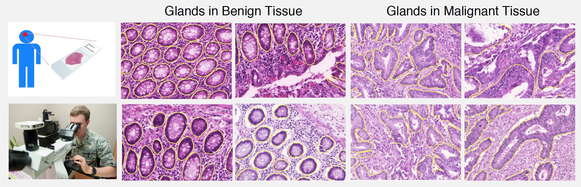
For adenocarcinomas, tumors originating in glandular structures of epithelial tissue such as prostate, pancreatic, and colorectal cancers, the differentiability of glandular architecture in histopathology images conveys significant information about the presence and degree of malignancy.
Here, we investigate a new set of features for quantifying the glandular architecture based on two recently developed persistent homology representations called persistence images [1] and persistence landscapes [2] and show their effectiveness in automated colorectal cancer diagnosis.
Brief background on persistent homology
In this section, we present a brief background on some fundamental concepts of persistent homology and the two recently proposed vectorized persistent homology representations: persistence image and persistence landscape.
- Given a point cloud dataset, persistent homology can be seen as a theoretical tool to detect and characterize prominent topological features (e.g. connected components, loops, voids) at multiple scales [3].
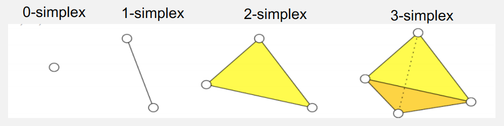
- Simplex: A p-simplex σp is defined as the convex hull of p+1 affinely independent points / vertices. A face of a simplex is defined as a subset of its p+1 points/vertices.
- Simplicial complex: A simplicial complex K is a finite collection of simplices. If a simplex is in K then all its faces are in K. Given a simplicial complex K, a simplicial complex L formed by a subset of its simplices is referred to as the sub-complex of K denoted as ?⊂?.
- Filtration: A nested sequence of simplicial complexes ? ⊂ ?1 ⊂ ?2 ⊂ ⋯ ⊂ ?n = ? is called a filtration of K.
- Homology groups: A d-dimensional homology group Hd(K) of a simplicial complex K is the set of all d-dimensional voids in K and the rank or number of these voids is referred to as the d-dimensional Betti number ?d(?).
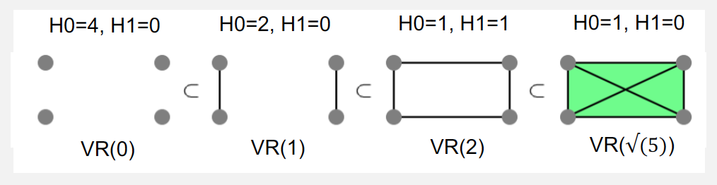
- Vectoris-Rips Filtration: Given a pointset, a simplicial complex VR ? = {? ∣ ???? ? ≤ ?} containing simplices of all subsets of its points whose max distance < ? is called a Vectoris-Rips (VR) complex. An increasing sequence of diameters/scales ?1 < ?2 < ⋯ < ?n results in a nested sequence of VR complexes ??(?1) ⊂ ??(?2) ⊂ ⋯??(?n) known as the Vectoris-Rips (VR) Filtration.
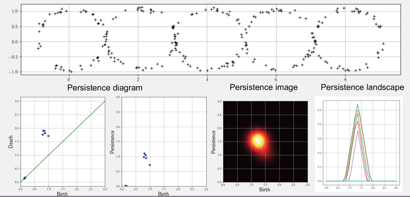
- Persistence diagram: Given a filtration F, the idea of persistent homology is to track the scales at which each d-dim void appears/disappears as a multiset ??d = {(?i, ?i)} of birth-death scales. Plotting them as 2D points produces the persistence diagram (PD) representation.
- Persistence image: Given a multiset of birth-persistence values ??d(?)={(?i, ??)} of all d-dim voids, the persistence image (PI) representation is generated by discretizing a 2D real-valued function defined as a weighted sum of bivariate gaussian PDFs centered at each birth persistence pair as follows:
- Persistence landscape: Given a multi-set of birth-death pairs { (bi, di) } with a triangular shaped function ?i(?) that linearly increases from (bi,0) to ( (bi+di)/2, (bi+di)/2 ) and then linearly decreases until (di, 0), the persistence landscape is defined as a 2D function ?:? ? ?→[0, ∞] where ?(?,?) is k-th largest value of of { ?i(x) }.
Methodology
In this section, we present our approach for using persistence image and persistence landscape representations to characterize the glandular epithelium architecture and train a machine learning model for cancer diagnosis.
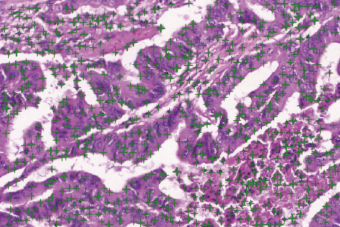
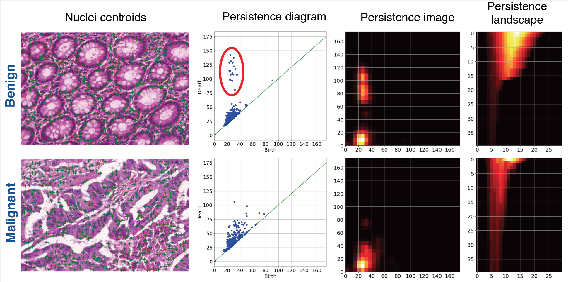
- Detect nuclei centroids: Given a histology image, we first pre-process it using the color normalization method of Reinhard et al [9] to standardize the staining. Next, we use the unsupervised color deconvolution method of Macenko et al [9] to extract the nuclear stain and apply minimum cross entropy thresholding [10] to segment the nuclear foreground. Lastly, we use a fast Difference-of-Gaussian implementation of a scale-adaptive Laplacian-of-Gaussian of Al-Kofahi et al [11] filter to detect nuclei centroids. The aforementioned pipeline of methods were developed using their implementations in HistomicsTK an open-source Python toolkit for histopathology image analysis that we are actively developing.
- Extract persistence homology features: Considering the set of nuclear centroids as a point cloud, we compute the persistence diagram of its Vectoris-Rips filtration for the homological dimension-1 corresponding to 2D loops using a fast multiscale approach developed by a researcher from Kitware named Samuel Gerber [6]. We then compute the persistence image (PI) and persistence landscape (PL) representations to characterize the 2D voids/loops formed by glandular epithelial cell nuclei and use them as features.
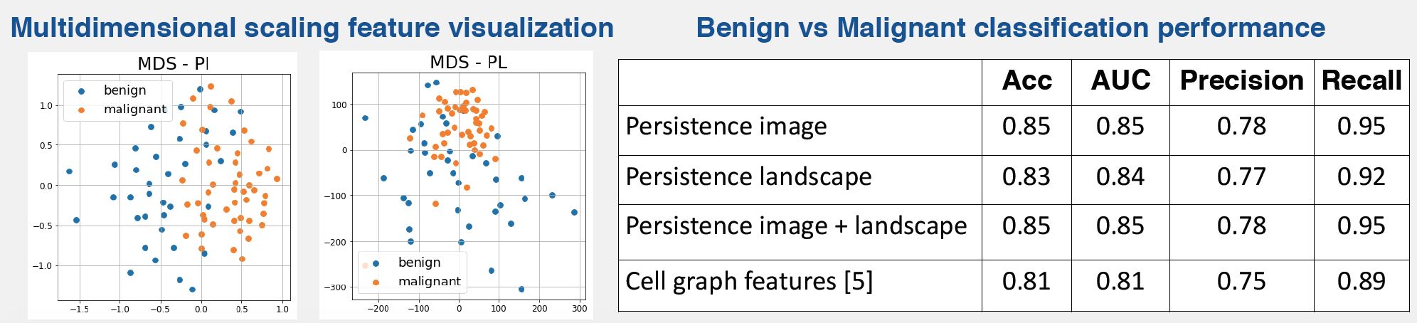
- Train machine learning model for cancer diagnosis: Given a training set of benign/malignant images, we train a random forest classifier based on the aforementioned features. We use principal component analysis (PCA) to reduce the dimensionality of each feature group such that 99% of the variance is preserved.
Results
We used the MICCAI 2015 Gland Segmentation Challenge dataset [7] to evaluate the proposed method. This dataset contains 165 images derived from 16 hematoxylin-eosin stained sections of normal and stage T3/T4 colorectal adenocarcinomas digitized using a Zeiss MIRAX MIDI SlideScanner at 20X magnification. An expert pathologist delineated the boundary of all the glands in each image and classified it as benign or malignant based on the overall glandular architecture. The dataset was divided by the challenge organizers into two parts: 85 training images (37 benign, 48 malignant) and 80 test images (37 benign, 43 malignant).
Conclusion
Using persistence image and persistence landscape based features to characterize glandular architecture in colorectal tissues, we were able to classify between benign and malignant images with a high degree of accuracy. Our preliminary experiments indicate that the performance of these features is better than state-of-the-art features based on cell graphs. Considering the vectorized nature of persistence image and landscape representations, we are currently evaluating their effectiveness in a deep learning setting.
For those who seek to leverage our expertise in developing algorithmic solutions to solve complex analytics problems similar to the ones described in this post, Kitware offers consulting and support services to help tailor our solutions to address user specific needs, create custom software, and/or conduct R&D. To learn more about the services offered by Kitware please contact us at kitware@kitware.com.
Acknowledgements
This work is funded by the NIH ITCR U24 grant U24-CA194362-01 entitled “Advanced Development of an Open-source Platform for Web-based Integrative Digital Image Analysis in Cancer” with Dr. David Gutman and Dr. Lee Cooper from Emory University as PIs and Kitware as a subcontractor.
References
- H. Adams, et al., “Persistence Images: A Stable Vector Representation of Persistent Homology,” JMLR, 18(1), 2015.
- P. Bubenik, “Statistical topological data analysis using persistence landscapes,” JMLR, 16(1), 2012.
- X. Zhu, “Persistent homology: An introduction and a new text representation for natural language processing,” in IJCAI, 2013.
- HistomicsTK – An open-source Python toolkit for histopathology image analysis https://github.com/DigitalSlideArchive/HistomicsTK
- S. Doyle, et al., “Automated grading of prostate cancer using architectural and textural image features,” in ISBI, 2007.
- S. Gerber, “Fast approximate multiscale persistence homology computation”, https://bitbucket.org/suppechasper/homology
- K. Sirinukunwattana, et al.,“Gland segmentation in colon histology images: The glas challenge contest,” Medical Image Analysis, 2017.
- E. Reinhard, M. Ashikhmin, B. Gooch, et al., “Color transfer between images,”IEEE Computer Graphics and Applications, vol. 21, no. 5, pp. 34–41, 2001.
- M. Macenko, M. Niethammer, J. S. Marron, et al., “A method for normalizing histology slides for quantitative analysis,” in IEEE International Symposium on Biomedical Imaging: From Nano to Macro, June 2009, pp. 1107–1110.
- H. Li and P.K.S. Tam, “An iterative algorithm for minimum cross entropy thresholding,”Pattern Recognition Letters, vol. 19, no. 8, pp. 771–776, June 1998.
- Y. Al-Kofahi, W. Lassoued, W. Lee, et al., “Improved automatic detection and segmentation of cell nuclei in histopathology images,”IEEE Transactions on Biomedical Engineering, vol. 57, no. 4, pp. 841–852, 2010