Virtual tour and high-quality visualization with ParaView 5.6 + OSPRay
Context
There are two common techniques in computer graphics to render surface geometries: Rasterization and Raytracing. By default, ParaView uses the Rasterization technique with OpenGL to display surfaces in real time but Raytracing is far better at rendering high-quality images.
ParaView 5.6.0 was recently released and includes a lot of improvements regarding OSPRay integration (see full release note here). OSPRay is an open-source raytracing renderer developed by Intel and highly optimized for CPUs. Two engines are available: sciviz and raytracer.
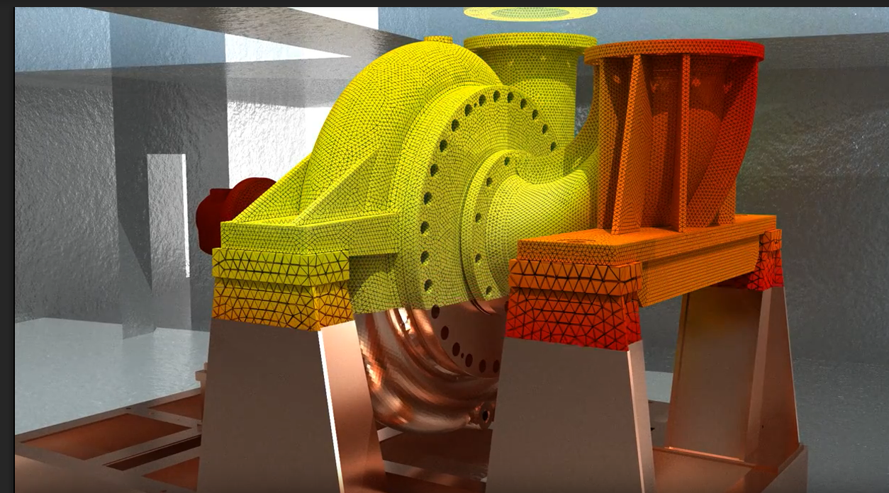
This blog post highlights the one specialized for realistic surface rendering – the raytracer engine – used to generate the following video. It shows a virtual visit of a power plant and shows that we can mix high-quality rendering and scientific visualization:
High-quality virtual tour of a power plant room with ParaView 5.6 and OSPRay. Data are (c) EDF.
Simulation credits: Modal analysis of a pump with code_aster.
According to an engineer of EDF: “A way to make accessible simulation results to non-expert audience is to render generated datasets into their real environment. In this context, OSPRay high-quality rendering is part of valuable tools for EDF to strengthen the comprehension of complex phenomena computed by simulation codes.”
OSPRay renderer allow mixing realistic rendering with scientific visualization.
The making of
OSPRay engine supports a lot of materials going from Metal to Glass in order to efficiently render all the materials you can find in the real world.
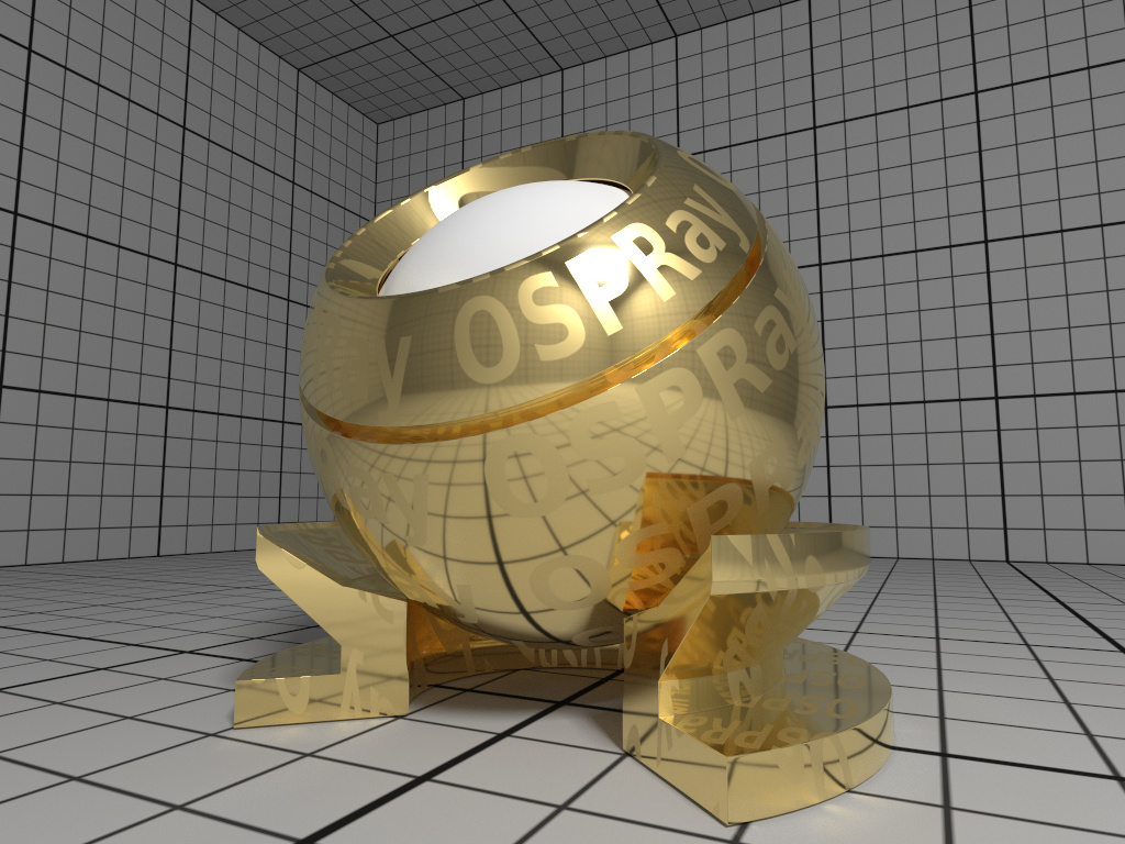 | 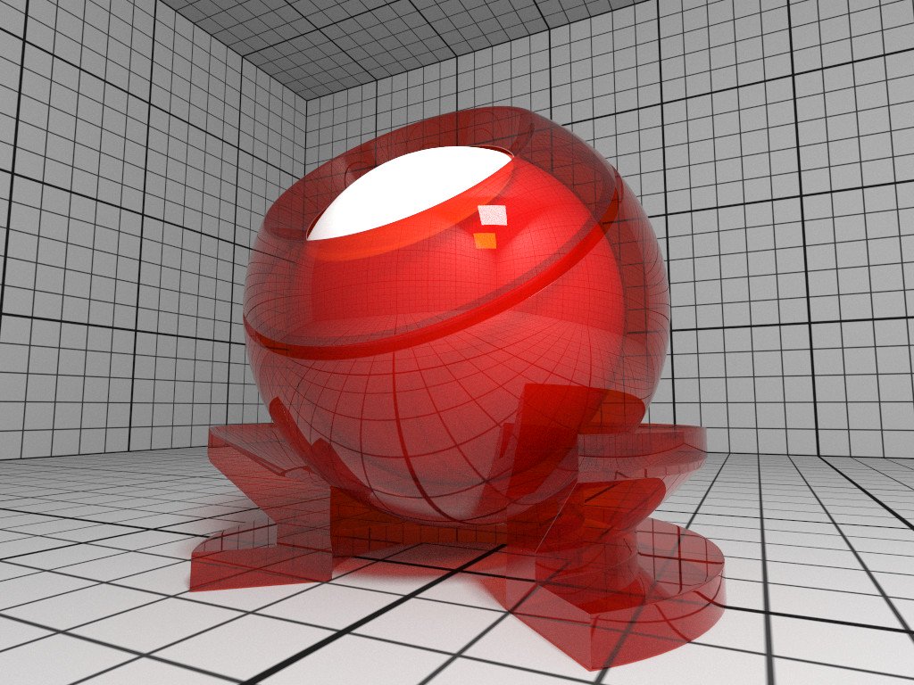 |
Examples of materials supported by OSPRay.
In ParaView, materials have to be defined with a JSON file and loaded in ParaView through the “File / Load OSPRay Materials…” menu.
Each material has different specific parameters, documented in the OSPRay documentation. It is important to have in mind that material properties can be uniform on the whole surface or declared through an external image acting as a texture. In the last case, the surface must have texture coordinates (and ParaView has several filters to compute such coordinates if needed). For example, the granular effect of the surrounding surface is created using a normal texture, transforming surface normal direction depending on texture coordinates:

Normal texture used to create a granular effect.
In our video, we used four different types of materials, depicted in this image:
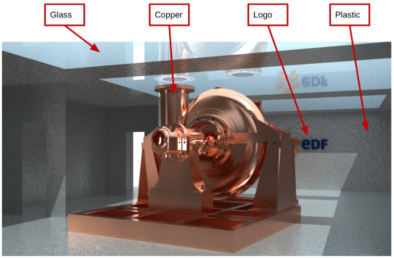
Annotation of the four different materials.
As an example, here is the JSON file used to setup those materials:
{
  "family" : "OSPRay",
  "version" : "0.0",
  "materials" : {
      "copper": {
          "type": "Metal",
          "doubles" : {
              "eta" : [0.1, 0.8, 1.1],
              "k" : [3.5, 2.5, 2.4],
              "roughness" : [0.2]
          }
      },
      "plastic": {
        "type": "Principled",
        "doubles" : {
            "roughness" : [0.2],
            "metallic" : [0.5]
        },
        "textures" : {
            "normalMap" : "plastic_base_Normal.jpg",
            "baseColorMap" : "plastic_base_Base_Color.jpg"
        }
      },
      "logo": {
        "type": "OBJMaterial",
        "textures" : {
            "map_Kd" : "logo.png"
        }
      },
      "glass": {
        "type": "ThinGlass",
        "doubles" : {
            "attenuationColor" : [0.85, 0.95, 1.0]
        }
    }
  }
}
The video contains 600 high definition images (1920×1080 pixels), with a high density of rays (300 samples per pixel) in order to completely eliminate the noise. This represents roughly 600 millions primary rays for each image!
For information, the video took approximately 35 hours to be generated with ParaView 5.6.0 on a distant headless Google Cloud compute node with 72 vCPU without GPU (OSMesa enabled).
Acknowledgments
This work was supported by EDF (Electricité de France)
Video and developments were done by Kitware SAS, France
Fantastic video and images! Excellent combination of scientific visualization and photorealistic rendering.
really nice video! I can see from the video that areas of high curvature the mesh edges are visible, how would you smooth those out?
Cells on the surface (triangles) are disjoints on purpose. In order to to smooth the surface, they have to be stitched (using the filter Clean) and you have to compute normals (using the filter Generate Surface Normals)
Great example. Thanks for sharing.
I have a plane with bump-mapped normals. Your “plastic” material declares a “normalMap” field with a jpg image, but I wonder if I could tell OSPRay to directly use my Normals since they are already properly bump-mapped?
Hi Jean,
In order to render a plane efficiently, four points and two triangles are enough. Of course, having bump-mapped normals on only four points will not be sufficient. That’s why using a texture is recommended and I think that OSPRay doesn’t support direct values on points for bump mapping.
I would recommend to generate a texture jpg image from your dataset : resample your plane to an image data and convert your normals to unsigned char RGB values (normalize the normals and map the range [-1.0;1.0] to [0,255] for each component).
Great video. Simulation credits: Modal analysis of a pump with @CodeAster, http://www.code-aster.org
Thanks. I have added the credits.